Post-processing calculations

RiverFlow2D has three output controls that make it easier for the user to analyze the results of the runs at specific sites in the domain calculator. These output controls are: Observation points, Cross sections and Profiles.

This tutorial illustrates how to incorporate the output controls in a model using the QGIS interface. The procedure includes the following steps:

1. Open an existing RiverFlow2D project.

2. Create ObservationPoints, CrossSections and Profiles layers, and draw the output controls.

3. Generate the mesh.

4. Running the model.

5. Review output files.

::: shaded The files required to follow this tutorial can be extracted from the 'ExampleProjects' zip file under the 'OutControlTutorial' folder. This zip file is downloaded separately from your installation materials. :::

Open an existing project

1. Open QGIS

2. On the Project menu click Open... and browse to the existing project: 'OutControlTutorial.qgz'.

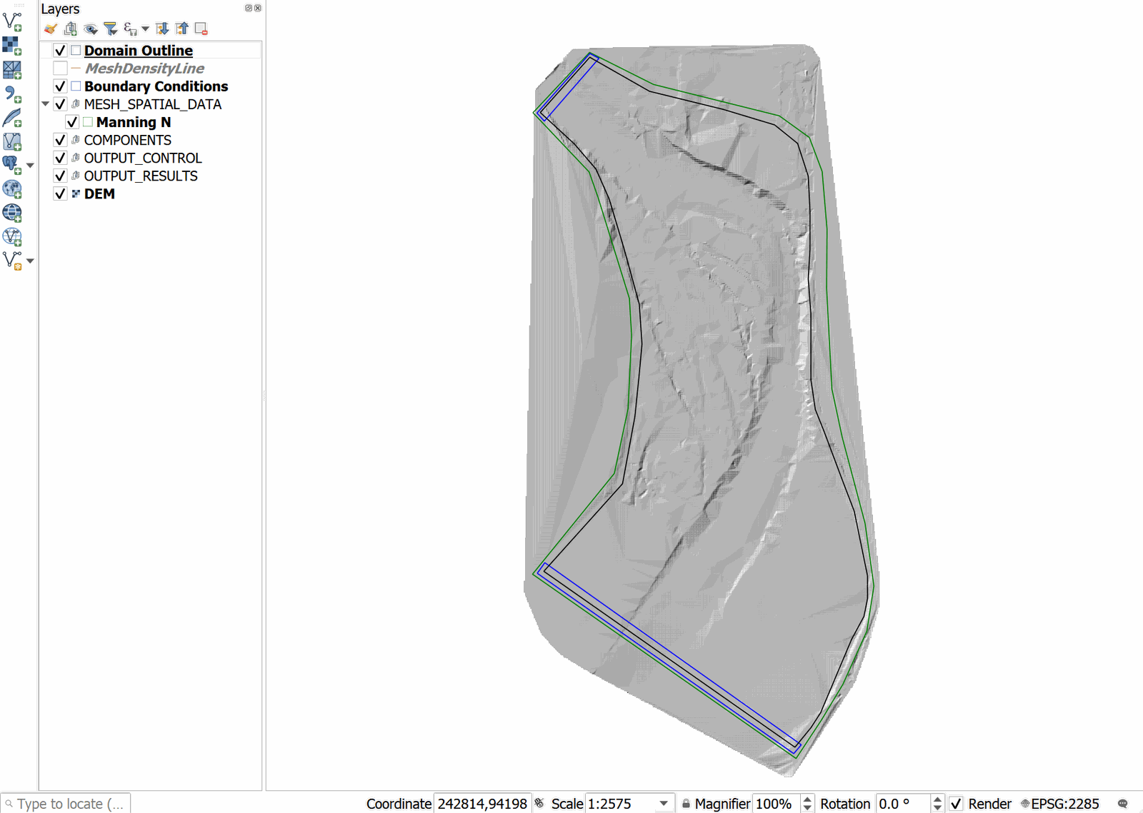
   This project contains the layers of the domain outline, the Digital Elevation Model DEM of the river bed in raster format, the layer with the boundary conditions where inflow is located in the upper left and outflow in the lower left. The boundary conditions are a hydrograph with a peak discharge of 6,500 \(ft^3/s\) and outflow condition set to Free outflow. When you open the project you will have an image of the project loaded in QGIS as shown in Figure 17.1.

   

Create a template of the layers ObservationPoints, CrossSections and Profiles and draw the output controls

To add the templates where the different output controls are drawn involves the following steps:

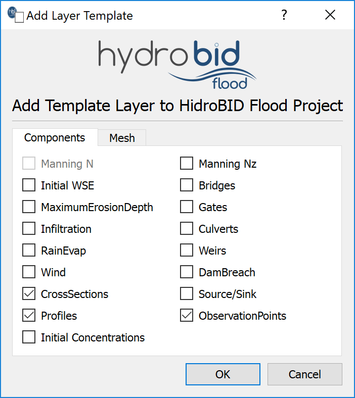
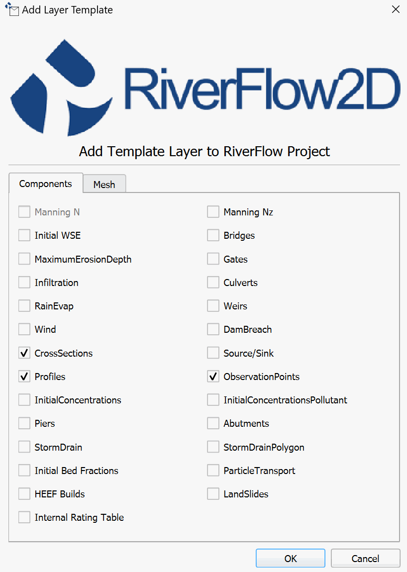
1. Create the templates of the layers ObservationPoints, CrossSections and Profiles: for this in the RiverFlow2D toolbar click on the New Template Layer button

   

   

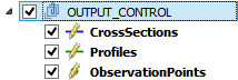
2. In the plugin window activate the checkBox ObservationPoints, CrossSections and Profiles, as shown in the Figure below:

   

   

3. Edit the layers and draw the output controls: Select in the layers panel, the ObservationPoints, CrossSections and Profiles layers one by one.

4. Click on the Toggle Editing button:

   

   A pencil will appear on the label of the layers, indicating that the layers are in edit mode:

   

5. Draw the lines or points that represent the output control: To draw the cross sections, profiles or observation points, the Add Feature tool will be used.

   for the CrossSections and Profiles layers, the icon for the Add Feature button is

   

   in the case of a point layer like ObservationPoints, the icon is

   

6. Drawing the cross sections: Select the CrossSection layer, and activate the Add Feature button.

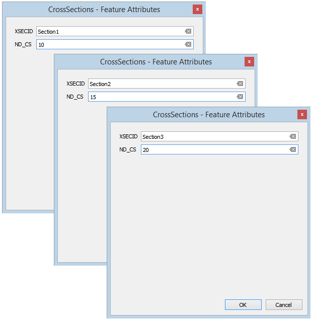
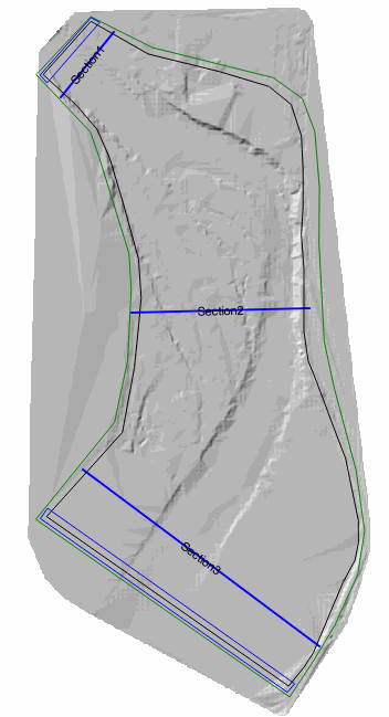
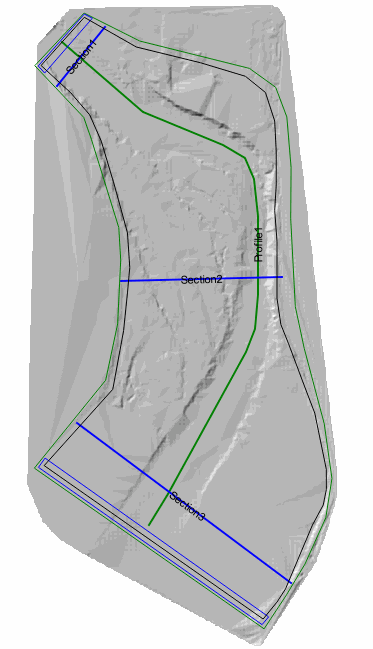
7. Proceed to draw three sections: One at the beginning of the channel, another in the middle and the third almost at the end of the channel, identify (XSECID) as: Section1, Section2 and Section3, with intervals (ND_CS) of 10, 15 and 20 respectively. The attribute tables of the sections will be as shown in Figure 17.4 and at the end of the drawing a similar image should appear as shown in the following Figure 17.5.

   

   

8. Save the polygon by clicking the Save button and click on the Toggle Editing button to deactivate Edit mode on the CrossSections layer.

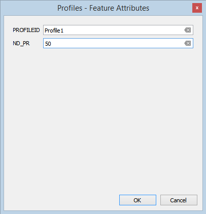
9. Drawing the Profile: Select the Profile layer and activate the Add Feature button, we proceed to draw the profile along the channel central axis, identifier (PROFILEID) is Profile1 and the number of intervals (ND_PR) equal to 50. The attribute table will be as shown in Figure 17.6. Once finished drawing, it should appear like the one shown in the following Figure 17.7.

   

   

10. To finalize the profile drawing, save the polygon by clicking the Save button and click on Toggle Editing button to deactivate Edit mode on the Profile layer.

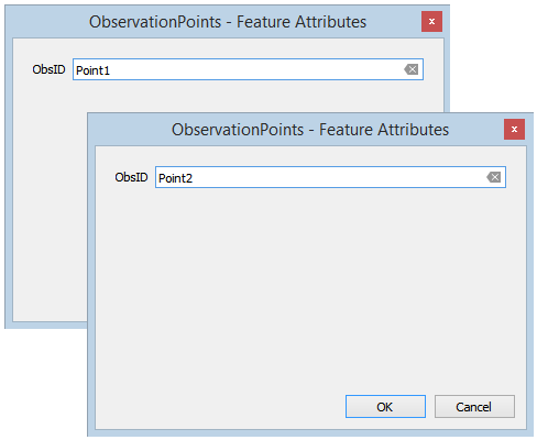
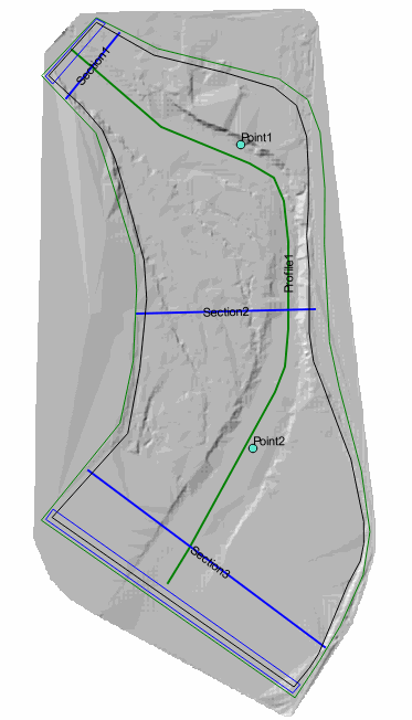
11. Drawing the observation points: Select the ObservationPoints layer, and activate the Add Feature button, proceed to draw two observation points, the first between sections 1 and 2 and the second between sections 2 and 3. As an identifier, (Obsid) is assigned Point1 and Point2 respectively. The attribute tables will be as shown in Figure 17.8 and at the end of the drawing you should have an image similar to the one shown in the following Figure 17.9.

    

    

12. To finish the drawing of the observation points, you click again on the Toggle Editing button to disable the editing mode of the ObservationPoints layer.

Generate the mesh

The mesh is generated with the Generate TriMesh button

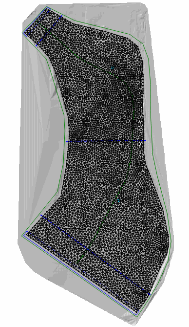
The result is a mesh of approximately 9,000 cells, as shown in Figure 17.10.

Exporting files to RiverFlow2D

Now that the mesh is generated and the other layers are ready with the necessary data, export the files in the format required by RiverFlow2D.

1. Click on the *Export RiverFlow2D * button

   

   

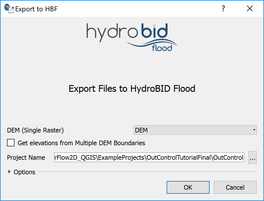
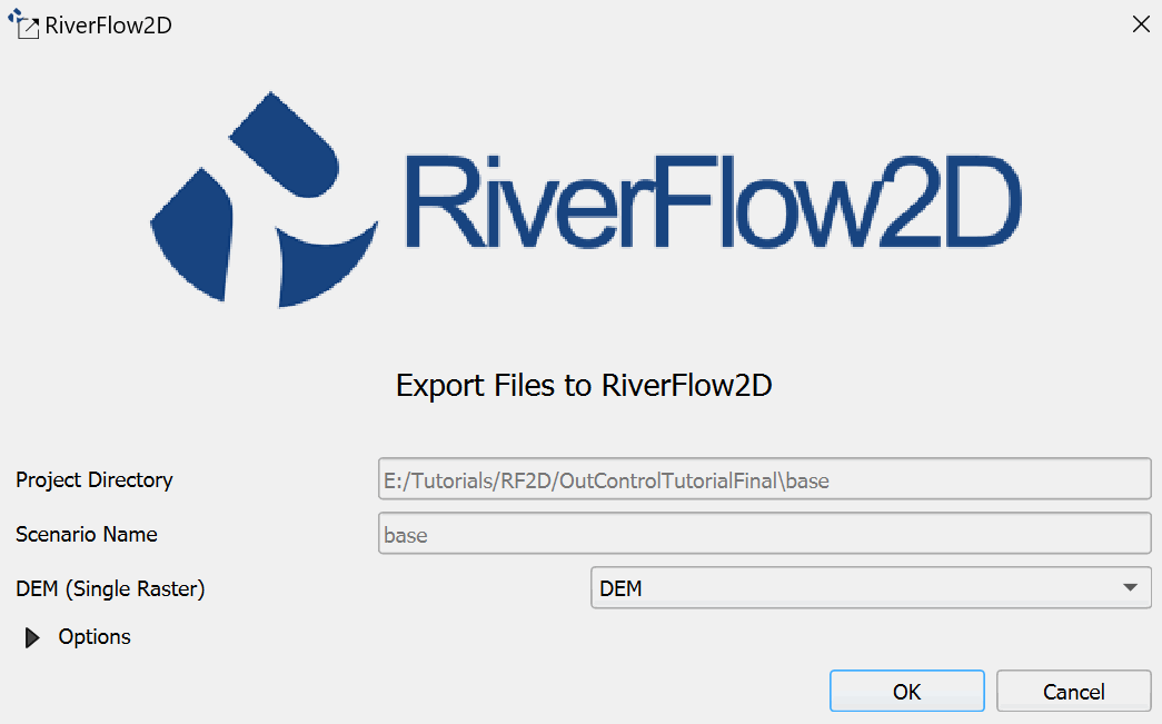
2. When run the plugin a window is displayed, select the raster layer that contains the Digital Elevation Model (DEM) and the name of the project to be exported.

3. Before executing the plugin, activate the layer with the DEM (if it is deactivated).

   Una vez ejecutado el complemento, se mostrara una ventana (Figura 17.11), como debe ser para nuestro ejemplo.

   

   

4. Once finished inputting the information, click the [OK] button to export the files to the model.

Once it is finished, RiverFlow2D will be loaded with the 'base.DAT' file.

Running the Model

After exporting the files, RiverFlow2D opens with the project file of the 'OutControl.DAT' sample and shows the Control Data panel to it as illustrated in Figure 17.13.

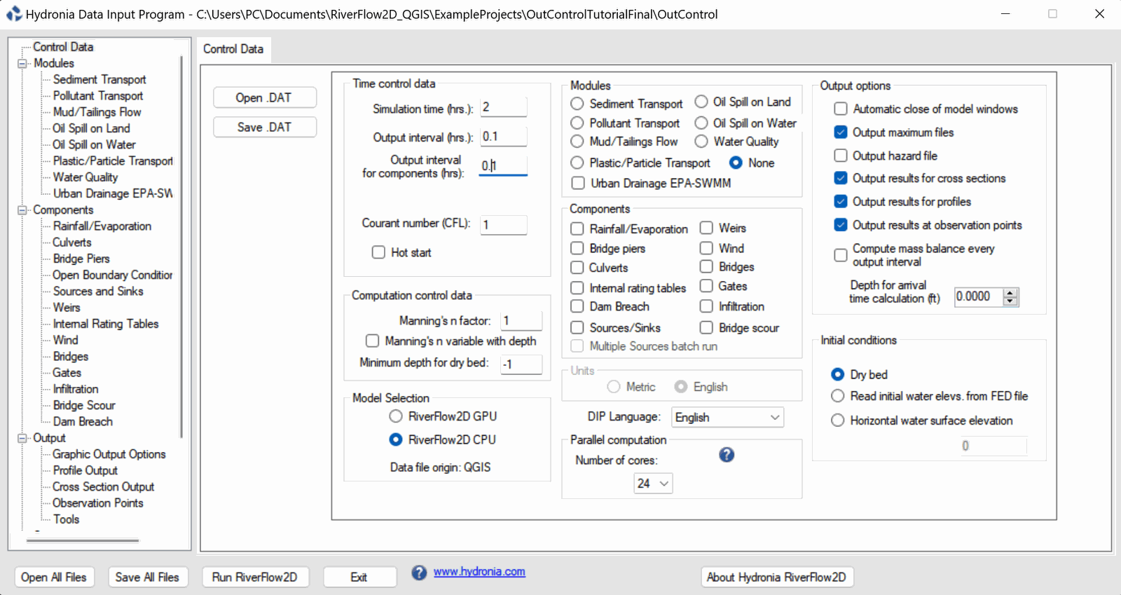
You can observe in the control panel in Output Options the outputs of results for Cross Sections, Profiles and Observation Points are selected.

Leave all other parameters at their default values.

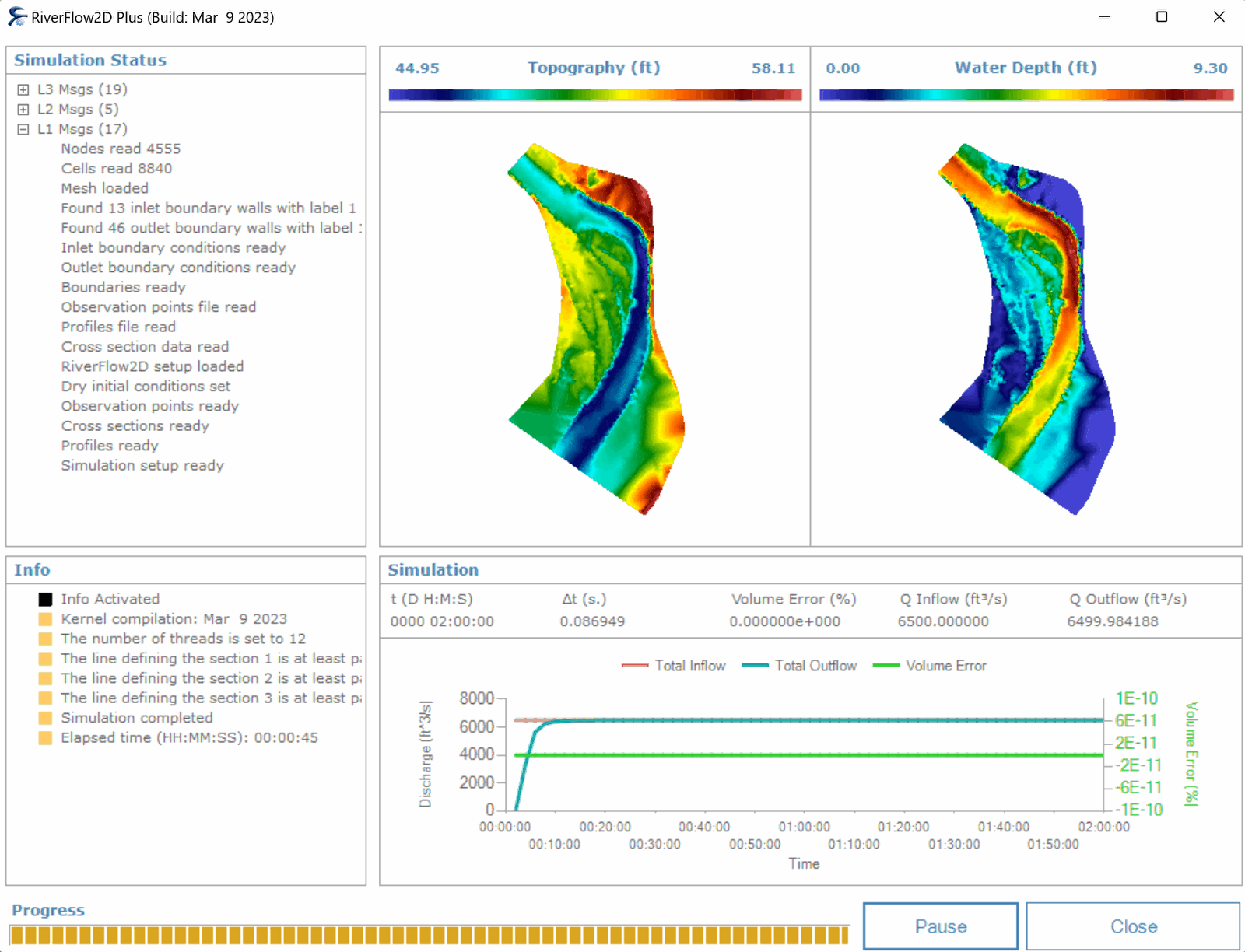
To run the model, click on the Run RiverFlow2D button. The window that RiverFlow2D presents while running the model shows: simulation time information, volume conservation error, total discharge of inflow in and outflow, as well as other parameters as execution progresses (Figure 17.14).

Review the output files

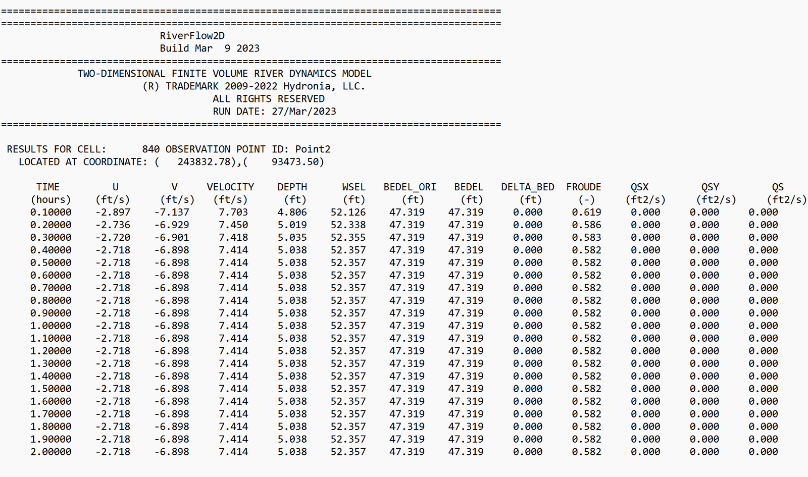
RiverFlow2D generates the files with the extensions '.xseci' (metric units) and '.xsece' (English units) which report the results along the cross sections. it generates files with extensions '.prfi' (metric units) and '.prfe' (English units) which report the results along the profiles and generates the files with the extensions '.outi' (metric units) and '.oute' (English units) that report the results in the observation points.

Figure 17.15 shows an extract of the 'OutControl.xsece' file with results at the cross sections:

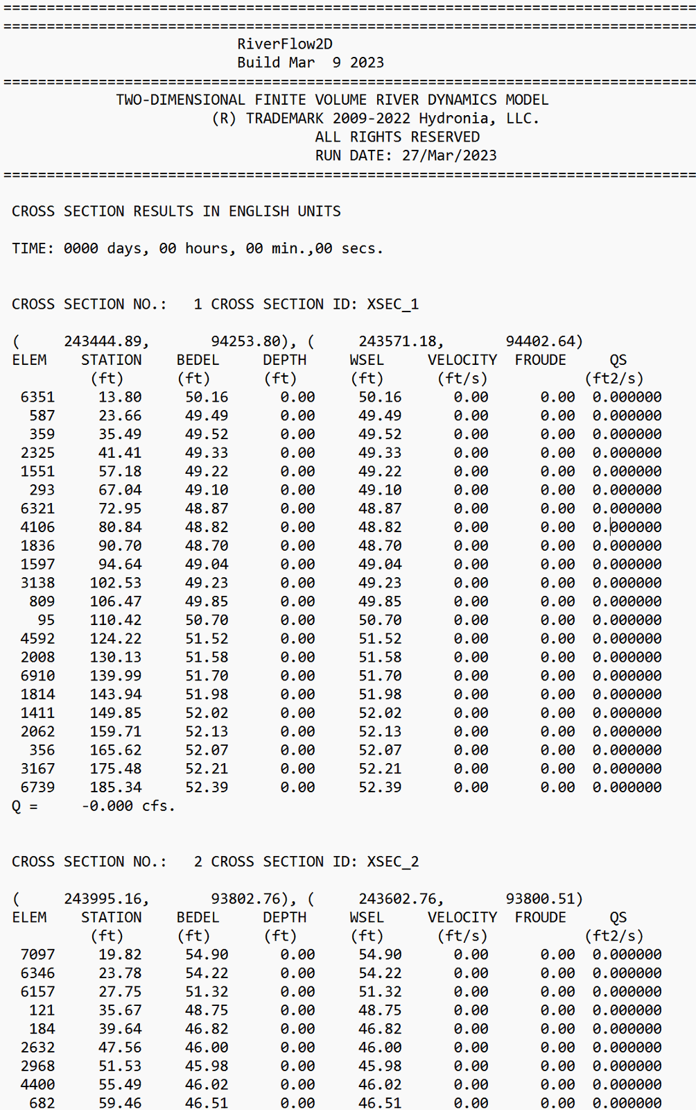
Figure 17.16 shows an extract of the 'OutControl.prfe' file with the report of the profile results:

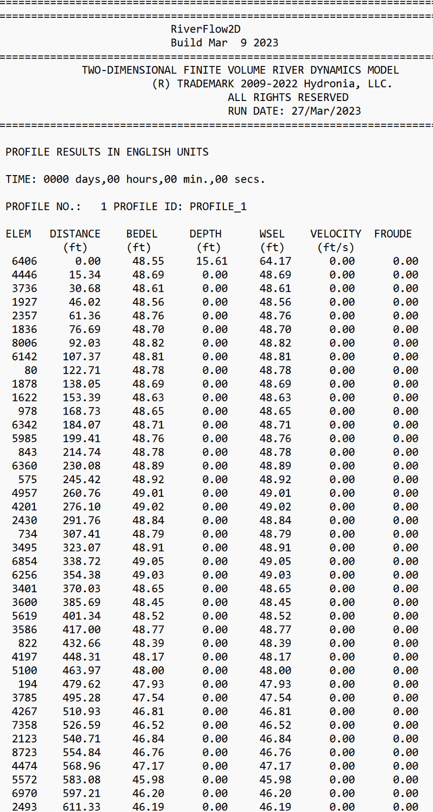
Figure 17.17 shows an extract of the 'RESvsT_Point1.oute' file with the report of the results of the observation point Point1: