Simulating culverts¶

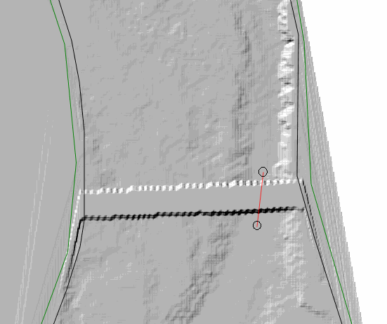
This tutorial shows how to incorporate culverts in an existing RiverFlow2D project using the QGIS interface. The problem consists of a natural channel crossed by a road embankment. A culvert structure is to be used to connect the upstream and downstream parts of the channel divided by the embankment as shown in the following figure:

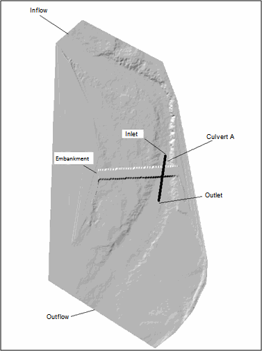
The water enters from upstream with a constant discharge of 1000 cfs, and outflows downstream along the indicated section. The area is initially dry. The culvert has a circular cross section, and other characteristics as summarized in the following Table (CulvertA). CulvertB data is provided in case that you wanted to extend the tutorial adding a second culvert to the project.

Parameter	Description	Culvert A	Culvert B Nb
Ke	Entrance Loss Coefficients	0.5	0.7
n	Manning's n Coefficient	0.014	0.015
Kp	Inlet Control Coefficient	0.3	0.4
M	Inlet Control Coefficient	2	2
Cp	Inlet Control Coefficient	1.28	1.1
Y	Inlet Control Coefficient	0.67	0.69
m	Inlet Control Coefficient	-0.5	-0.5
Dc	Diameter (feet)	3	2
-	Inlet Inverted elevation	-9999	-9999
-	Outlet Inverted elevation	-9999	-9999

The procedure to integrate this culvert into a RiverFlow2D simulation involves the following steps:

Open an existing RiverFlow2D project.
Add a Culvert component layer.
Draw the line of culvert alignment.
Input the data or attributes for the culvert.
Export the files to the RiverFlow2D program.
Running the model.
Review culvert output files.

::: shaded The files required to follow this tutorial can be extracted from the 'ExampleProjects' zip file under the 'CulvertTutorial' folder. This zip file is downloaded separately from your installation materials. :::

Open an existing project¶

Open QGIS.
On the Project menu click Open... and browse to the existing project: .

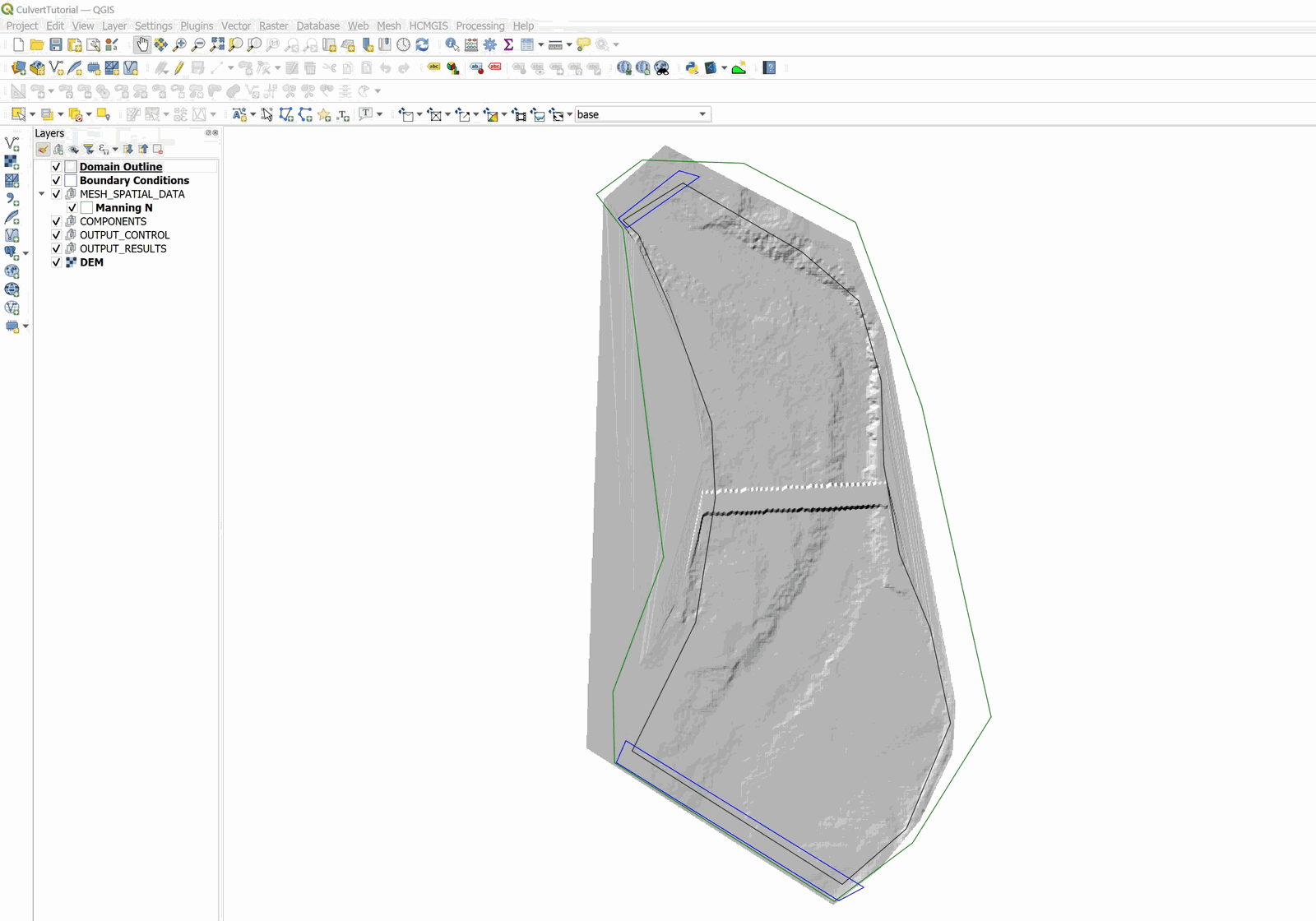
This project contains the following layers: Domain Outline, Digital Elevation Model (DEM) in raster format, polygon with the Manning's n coefficient, and the boundary condition polygons. The inflow is located in the upper left, and the outflow in the lower left. The boundary conditions corresponds to a constant discharge of 1000 \(ft^3/s\), and outflow conditions is set to free. Figure 6.2 shows the opened project.

Create Culverts layer and draw the culvert¶

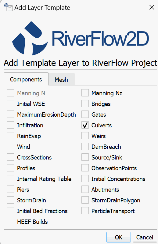
To create the Culverts layer, in the RiverFlow2D toolbar click on the New Template Layer icon
In the window select the Culverts checkBox, as shown:
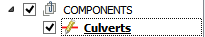
Edit the Culverts layer: In the layers panel select the Culverts layer and in the digitalization toolbar click on the Toggle Editing button

A pencil icon will appear in the Culverts layer indicating that the layer is in edit mode:
Draw the line representing the culvert alignment: Using the tool Add Feature from the digitalization toolbar

draw the line that represents the culvert. It is only necessary to indicate two vertices.
Right-click to finish drawing. You should get an image similar to the one shown in the following Figure:
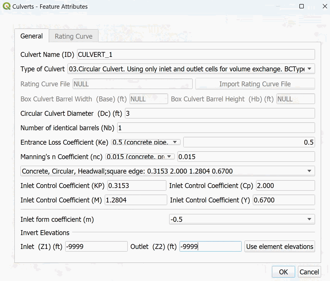
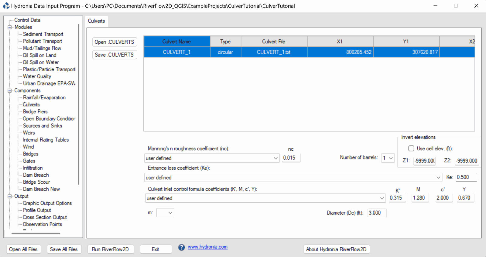
Enter the culvert data: After the culvert drawing is finished, the window to input the culvert attributes immediately appears. The dialog window has 2 tabs, in the General tab you enter the basic data for circular and box culverts:
- Culvert Name (ID): CULVERT_1,
- Type of culvert: Type 3 (Circular culvert)
- The rest of the parameters are coefficients that needed to compute the culvert discharge. To help with the introduction of these parameters, the window presents a list with default values for different types of culverts. If one of the values of the list parameters is not appropriate, you can choose the option where the value is defined by the user (user defined). The window of the culvert parameters should be similar to the one shown in the Figure below:
After inputting the values, click on the OK button.
Save the changes in the layer using the Save button of the digitalization toolbar
Disable the editing mode of the layer with the Toggle Editing button

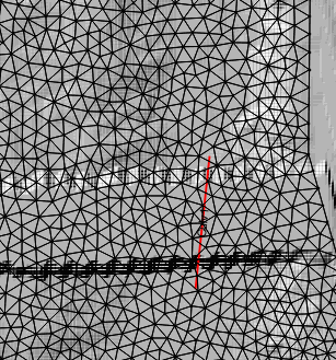
Generate the mesh¶

The mesh is generated with the Generate Trimesh tool

the results obtained as shown in Figure 6.6.

Exporting files to RiverFlow2D¶

Now that you have generated the mesh and you have the other layers ready with the necessary data, you should export the files in the format required by RiverFlow2D.

Click the Export RiverFlow2D button
The raster layer that contains the Digital Elevation Model (DEM) and the name of the scenario should already be set.

A window will appear as shown in (Figure 6.7).

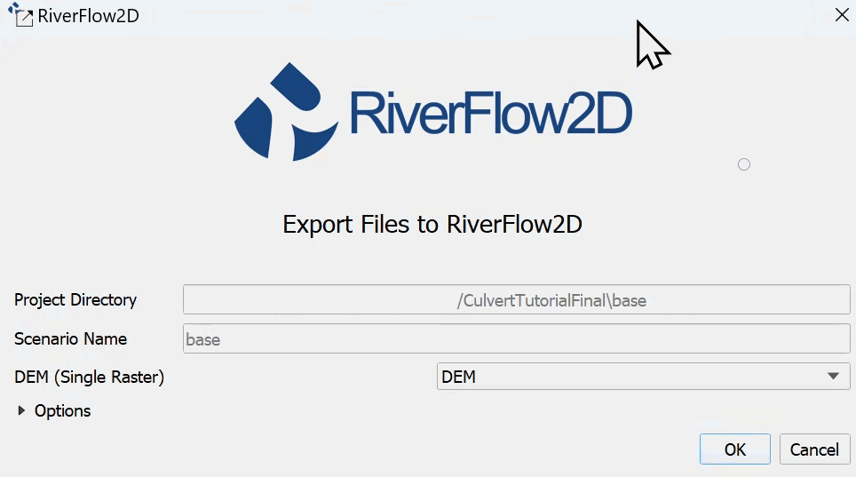
Once done reviewing, click on the [OK] button and the export process will begin. Once finished processing, the RiverFlow2D program will be loaded with the 'CulverTutorial.DAT' file.

Running the model¶

After exporting the files, the RiverFlow2D program is loaded with the project file from the 'CulvertTutorial.DAT' example and shows the Control Data panel to it as illustrated in Figure 6.8.

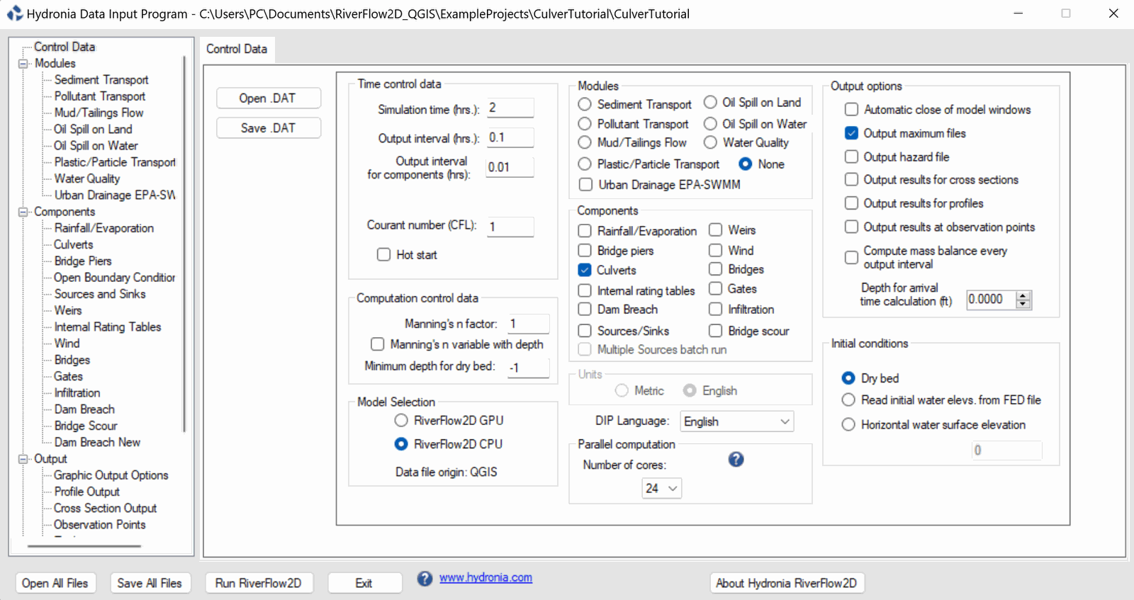
Note that the Culverts Component appears selected. On the left side of the Control Data panel, in the list of components select Culverts to activate the Culverts panel. The contents of the culvert file prepared by QGIS will be displayed (Figure 4.10).

Leave all other parameters at their default values.

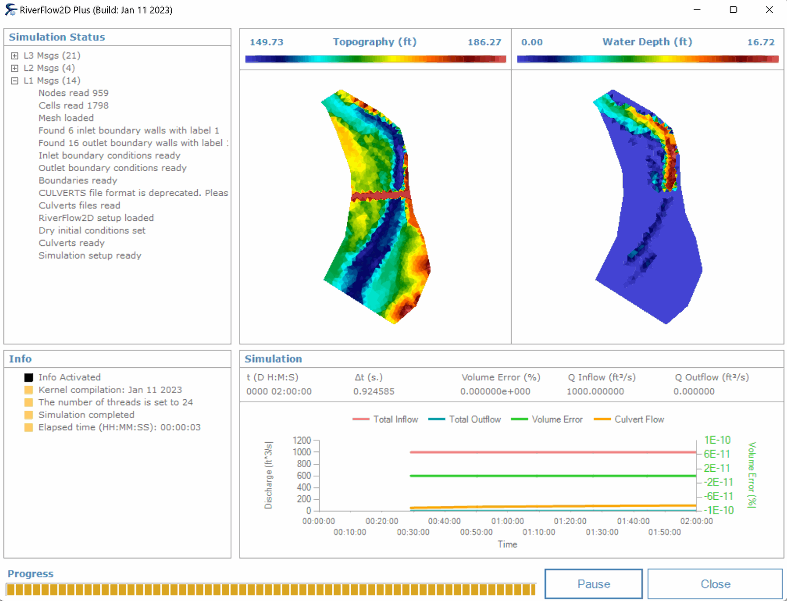
To run the model, click on the Run RiverFlow2D button in the lower section of Hydronia Data Input Program. A window will appear indicating that the model began to run. The window also reports the simulation time, volume conservation error, total input and output discharge, and other parameters as the execution progresses (Figure 6.10).

Review culvert output file¶

For each culvert, RiverFlow2D creates an output file called: 'CULVERT_culvertID.out', where 'culvertID' is the name (ID) entered when we created the culverts. Output includes the series of discharge versus time through the culvert and the elevations of the water surface at the inflow and outflow locations. For this tutorial, you will find a file called 'CULVERT_CULVERT_1.out', whose content is shown in the following figure:

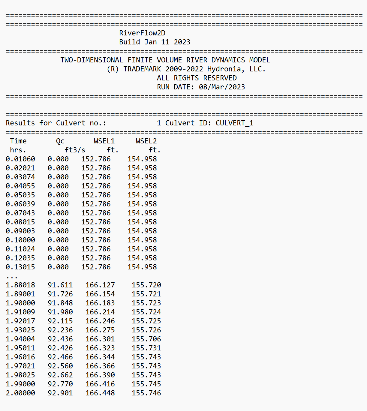
This concludes the Simulating culverts tutorial.