Creating high-impact graphics and animations using Paraview

ParaView is an open-source, multi-platform data analysis and visualization application. You can quickly build visualizations to analyze model results using qualitative and quantitative techniques. The data exploration can be done interactively in 2D and 3D, or using ParaView's batch processing capabilities.

This tutorial will demonstrate the use of Parview to generate high quality graphics, including depth maps, velocity fields, 3D visualizations, and animations of RiverFlow2D results.

::: shader This tutorial requires ParaView version 5.8.1 or later. You can download and install ParaView version 5.8.1 or later from the website www.paraview.org. To create the ParaView graphs, the RiverFlow2D model needs to generate during runtime the '.vtk' files using the Create graphic output files option in the Hydronia Data Input Program Graphic Output Options panel. :::

Paraview basics

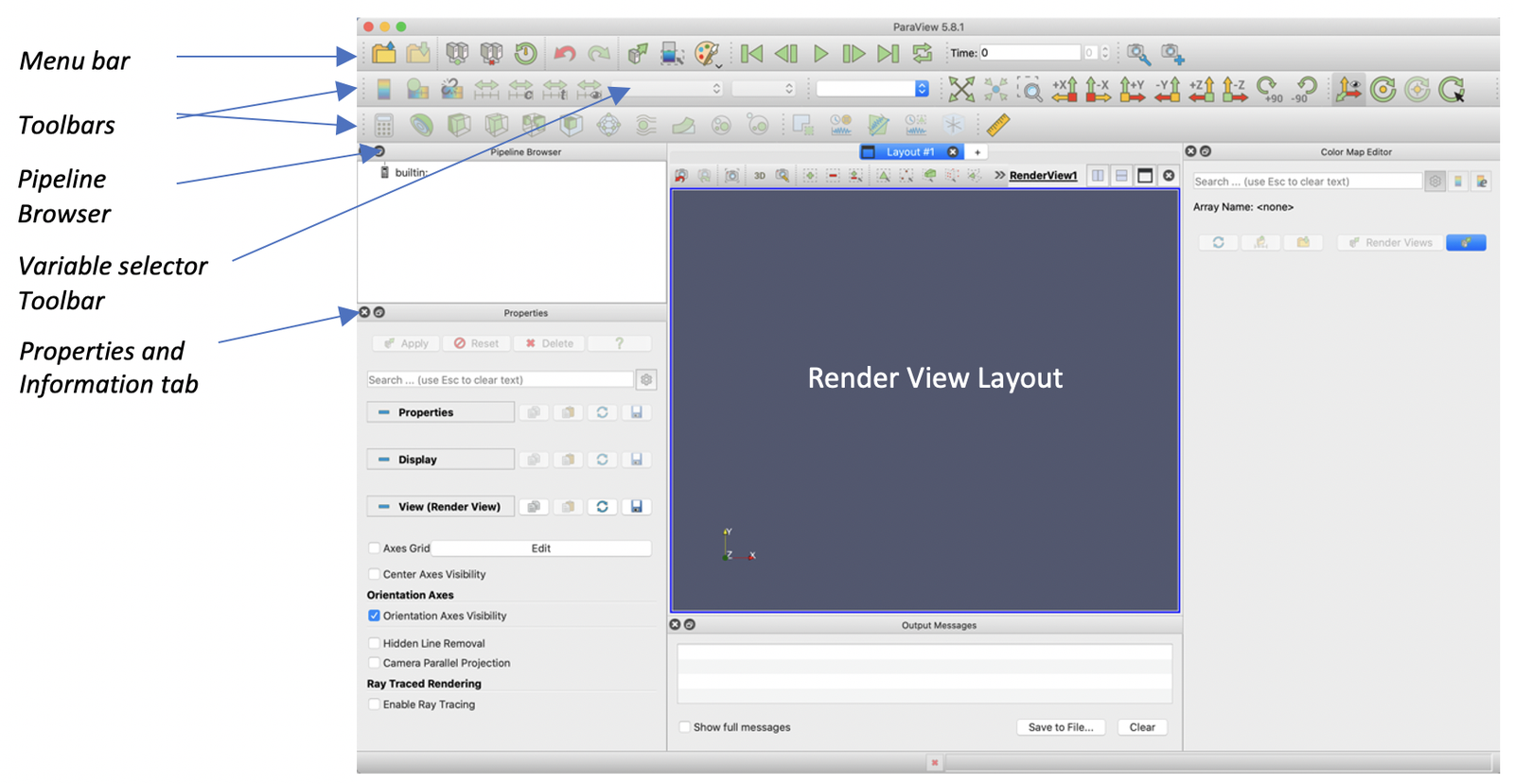
After loading Paraview, the following components can be identified in the main window (see Figure 21.1):

To open the tutorial example group file, click in the Menu bar and double-click the file group 'BridgeTutorial..vtk' in the 'ParavirewTutorial' folder. The group contains multiple '.vtk' files, where each file corresponds to a specific simulation time.

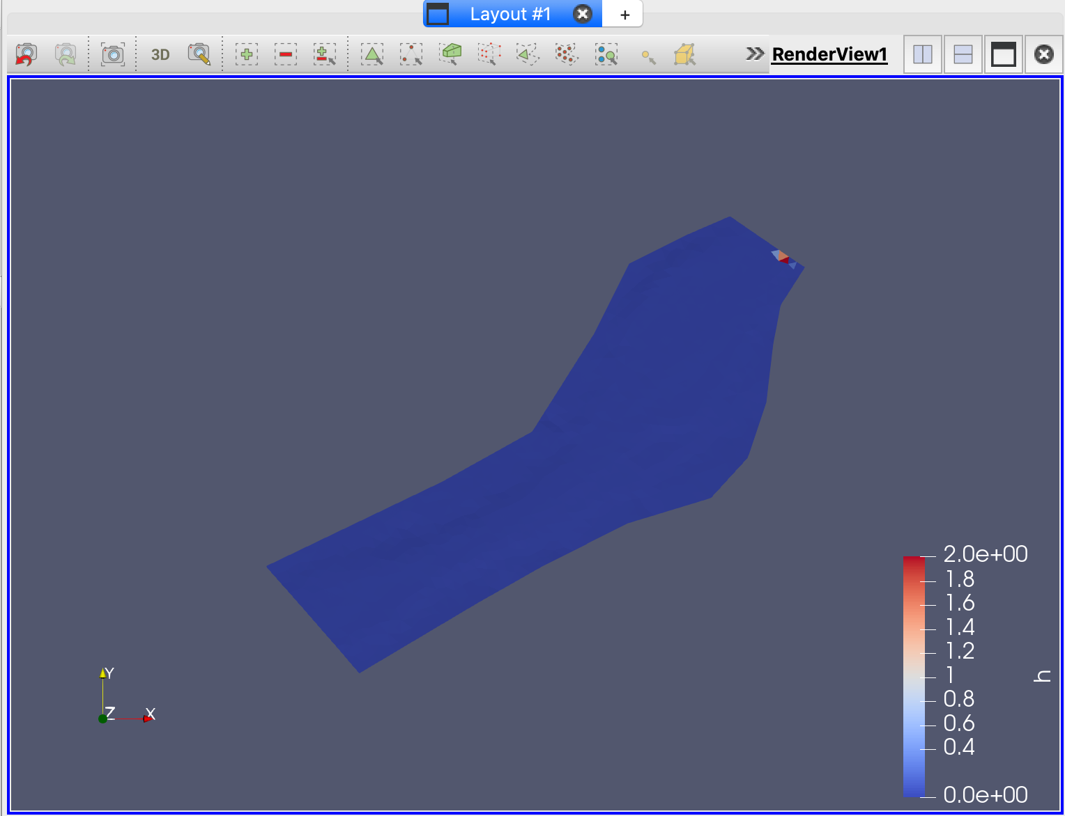
Make it visible clicking Apply in the Properties tab. The following graphic in the Render View layout will look as follows:

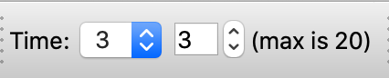
Using the Time control toolbar (see Figure 21.3), select a time to visualize the selected variable.

The graphic will change according with the selected simulation time. For example, for Time = 2 it should look similar to this:

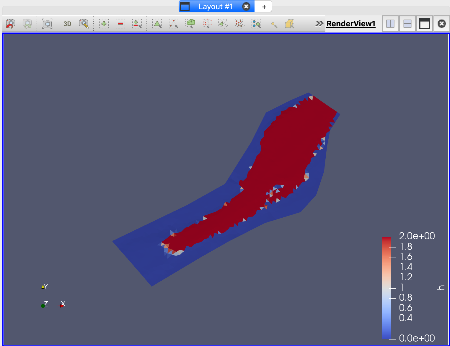
An adequate visualization depends on the selection of a color scale of a defined variable. In the previous figure, the default color scale was selected associated with the depth variable (h). The next section shows how to customize color rendering.

Two-dimensional (2D) visualizations

Create a 2D bed elevation map

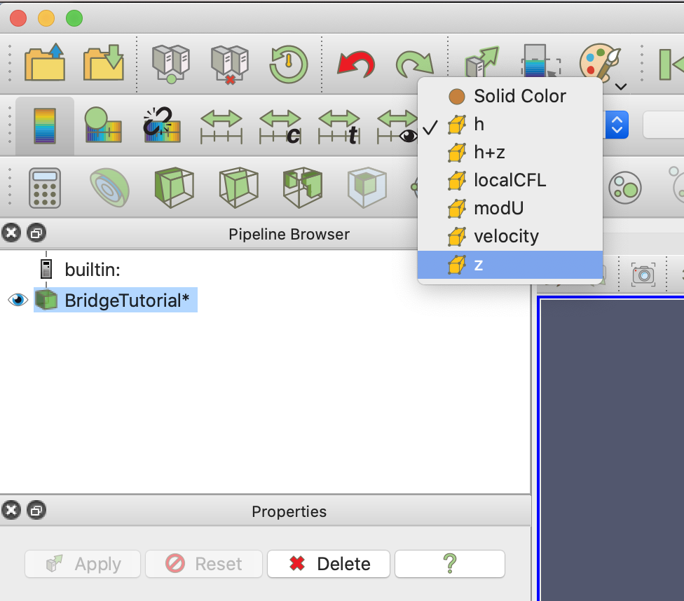
Paraview has many filters for full visualization of 1D, 2D and 3D data. In this part of the tutorial we will create a 2D bed elevation graphic. Select the bed elevation variable z in the Variable selector:

The representation of the bed elevation z will look like this:

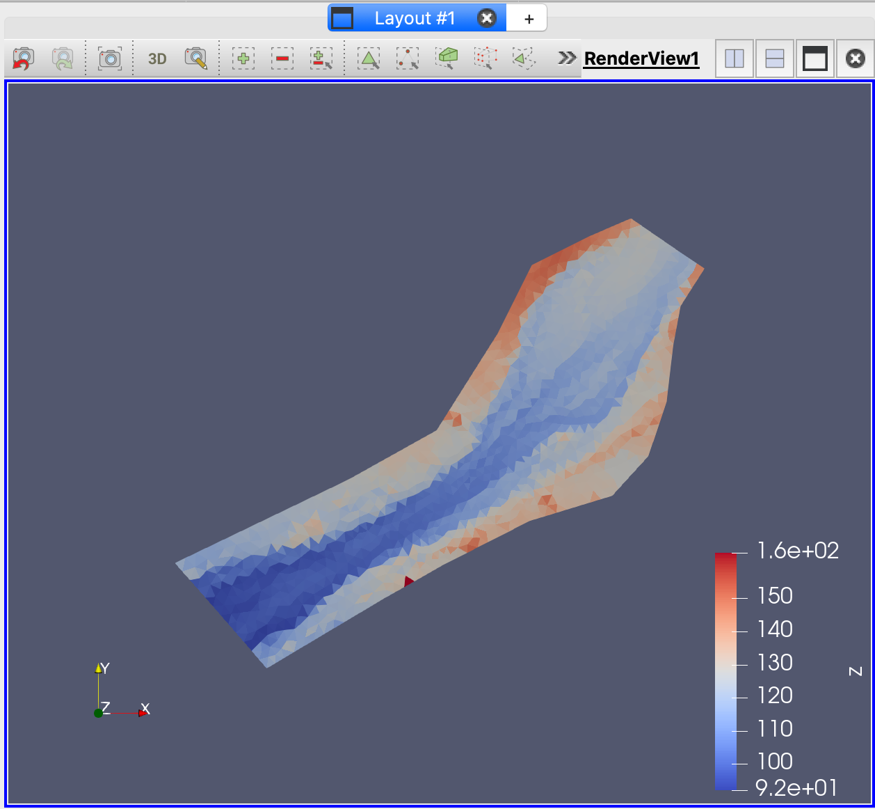
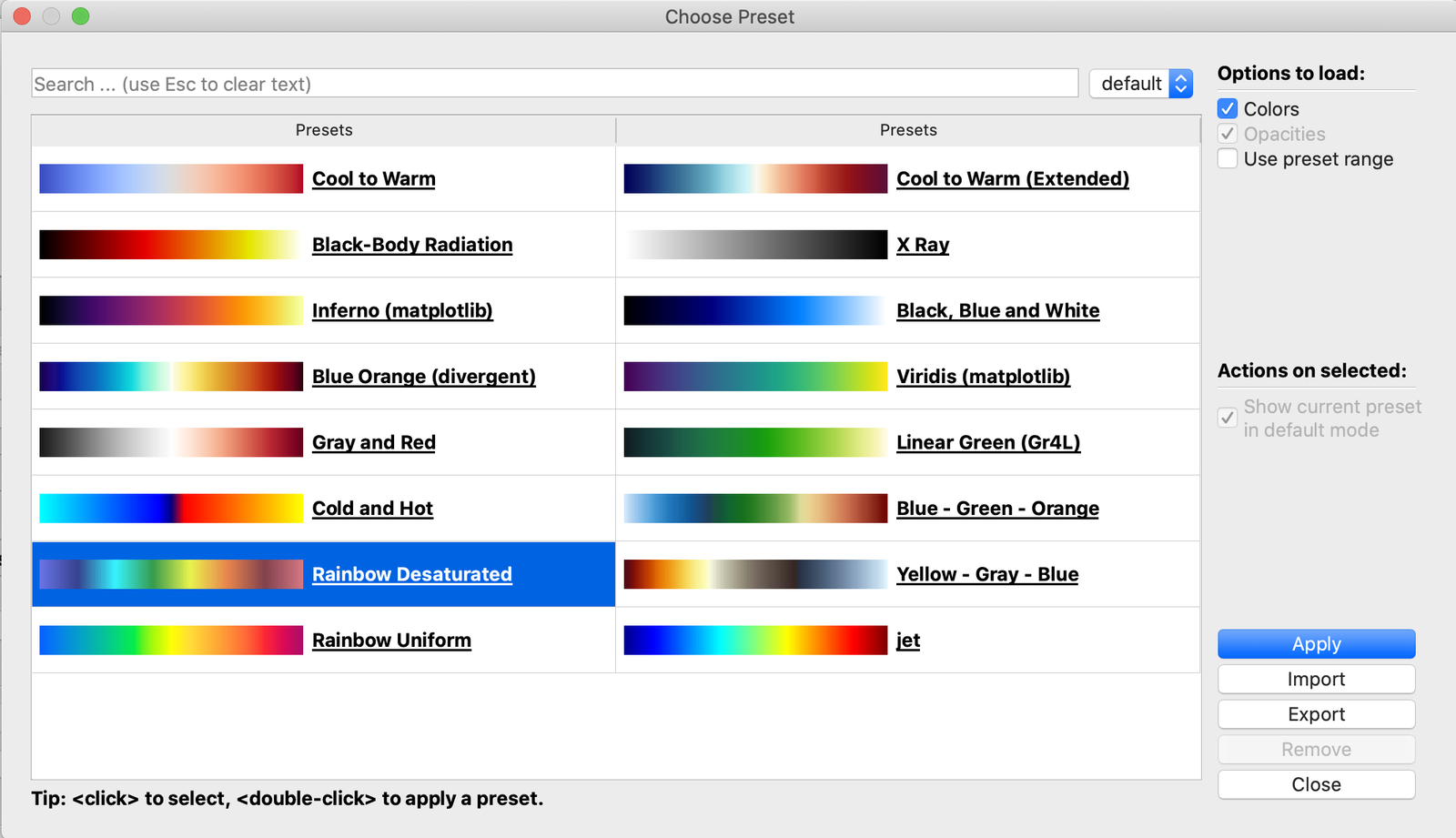
Although it is possible to customize the color maps, we will see how to do it later in this tutorial, for this example we will use a predefined color.

Click in the Properties tab to pick up the Rainbow Desaturated color map in the Choose Preset dialog box. Once selected, Apply/Close.

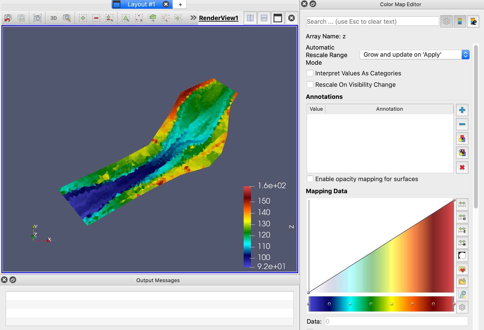
The result graph visualizes of the bed elevation z.

Creating 2D velocity vector fields

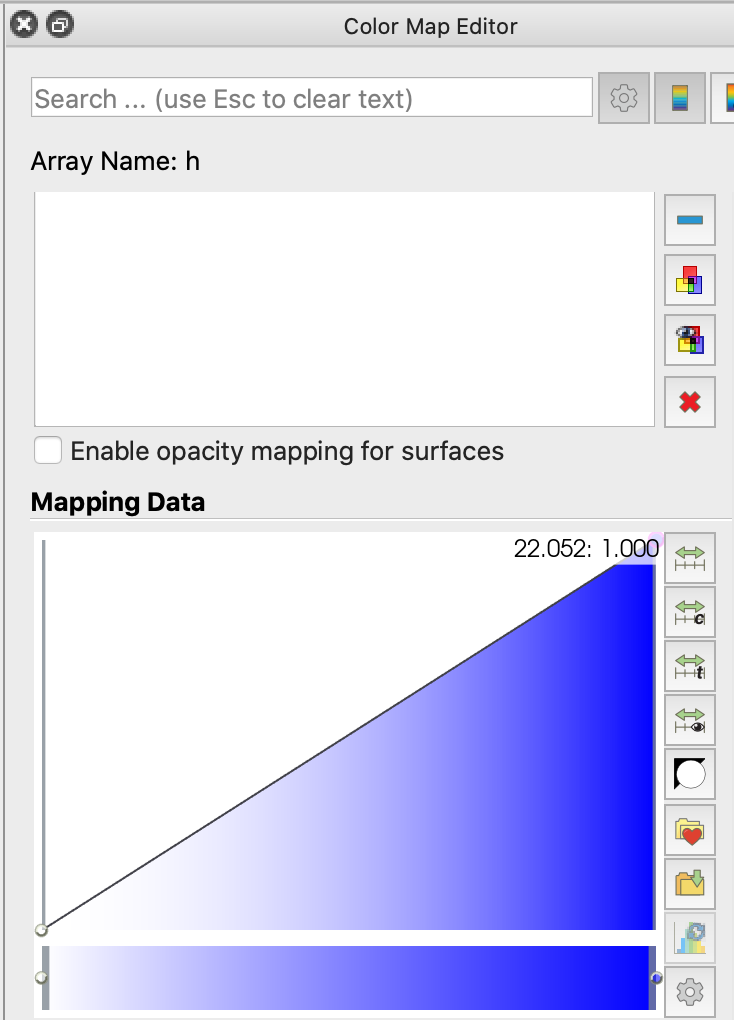
In order to create a 2D visualization of the flow and its magnitude with our project data, we will start with a water depth h representation in a white-to-blue color scale. The first step is to select h in the Variable selector. To change the color map for water depth h to a white-to-blue, click and choose the XRay preset color then Apply/Close. The Mapping Data should look as:

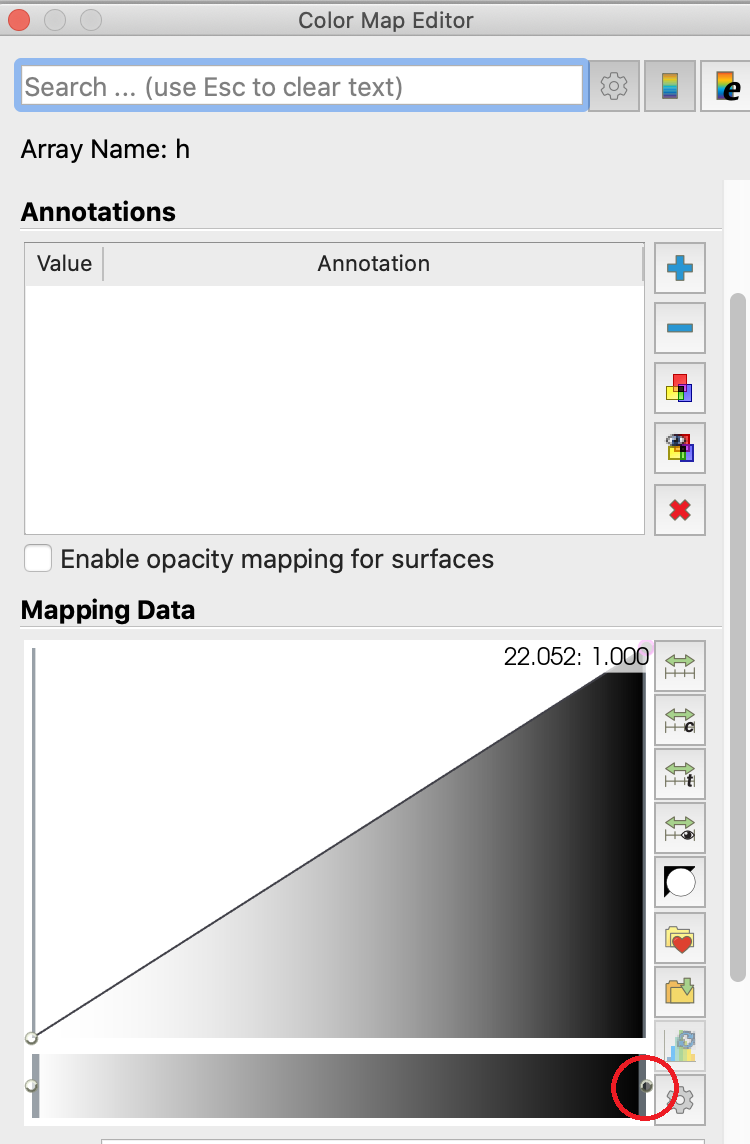
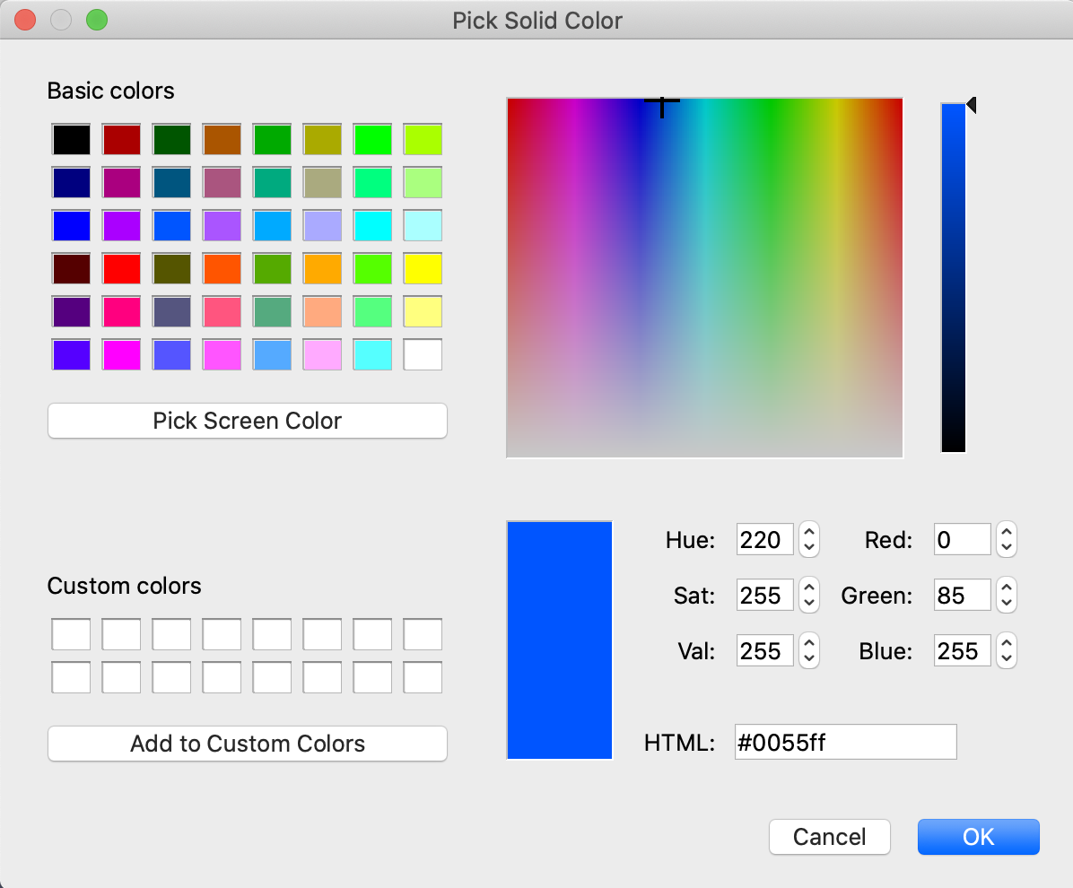
Double click in the right circle of the range marker bar and select any blue color from the Select Color dialog box. This example uses Red = 0, Green = 85 and Blue = 255 and Click OK

The Mapping Data will look as follows:

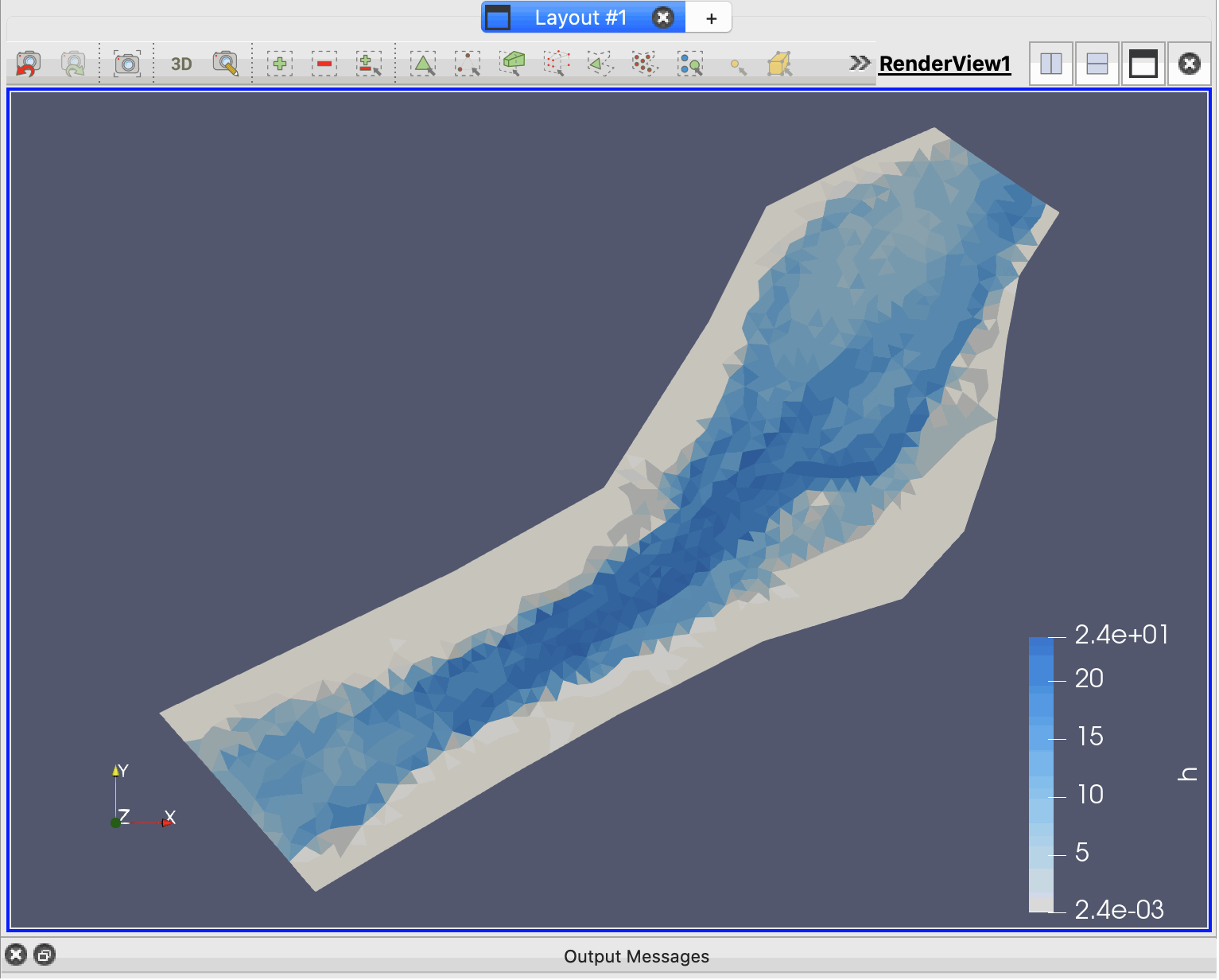
Set the Time = 20 and the result should look as follows:

To create a 2D velocity vector map for this example, follow these steps:

• Select BridgeTutorial* in the Pipelines Browser

• In the Filters menu select Common/Glyph

• Click Apply in the Properties panel. You will adjust the big arrows after

• Configure the Vector field configuration in the Properties panel as follows:

  • Glyph type: 2D Glyph

  • Scale Array: modU (velocity modulus)

  • Scale Factor: 35

  • Glyph mode: Every Nth Point

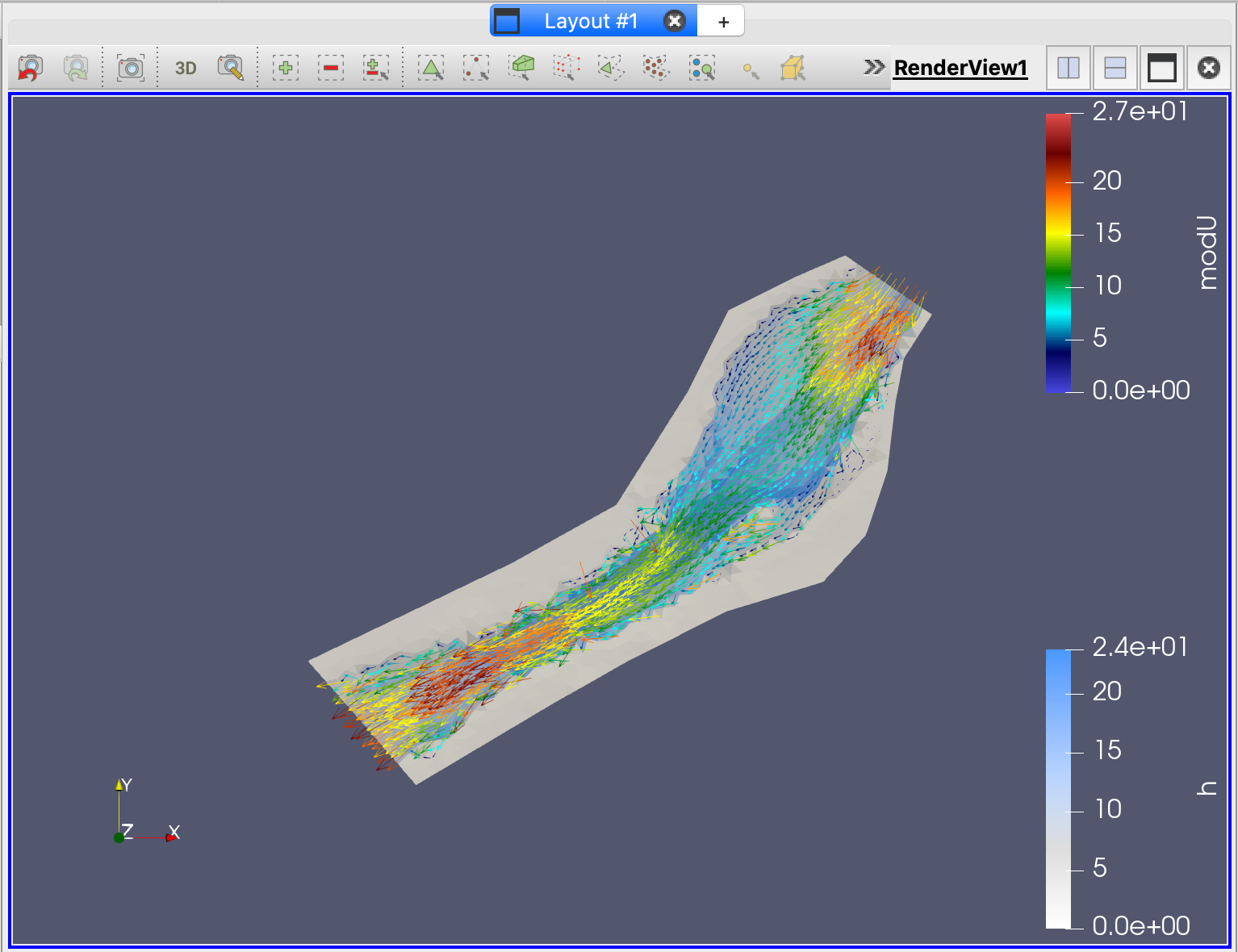
  • Click Apply to visualize the the filter setup. The user can press this button each time changes are made

  • Coloring: modU

• Choose the Rainbow Desaturated color scale clicking in and Apply/Close.

In order to save the Paraview project, select File/Save State. This will save a '.pvsm' file.

Three-dimensional (3D) visualizations

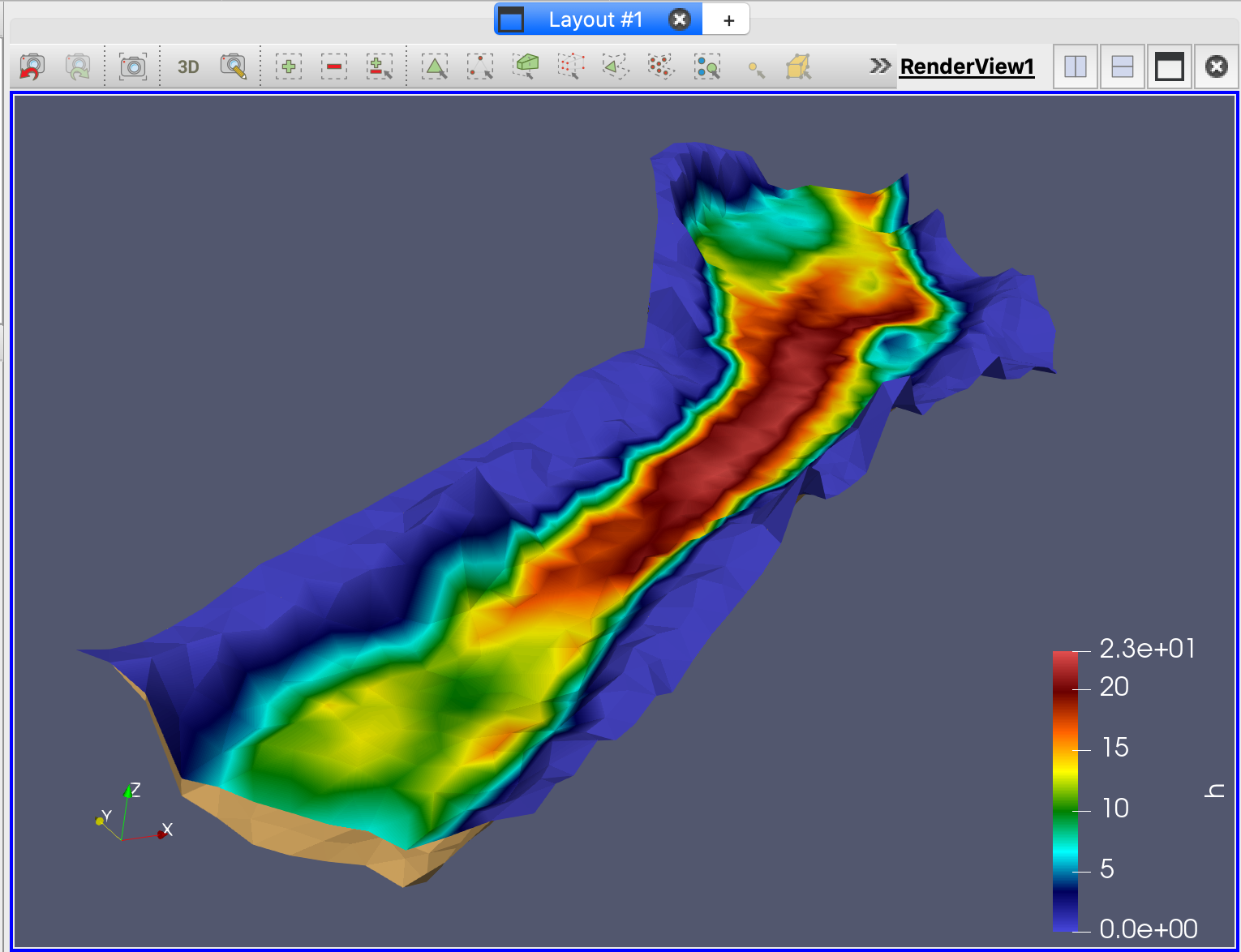
In this part of the tutorial we will explain the steps to create a 3D visualization using Paraview. We start where section 21.2 ends. This assumes that we have a visualization of the bed elevation (z) variable using the Rainbow Desaturated color map.

Open the 'BridgeTutorial..vtk' group as explained in section 21.1 and select the bed elevation variable z in the Variable selector. The render view should look as the following figure:

Generating a 3D visualization in ParaView requires an interpolation from Cell Data to Node Data as follows.

• Select Cell Data to Point Data in the Filters/Alphabetical menu. Then, press the Apply button in the Properties tab.

  

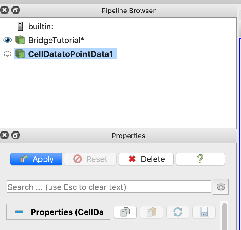
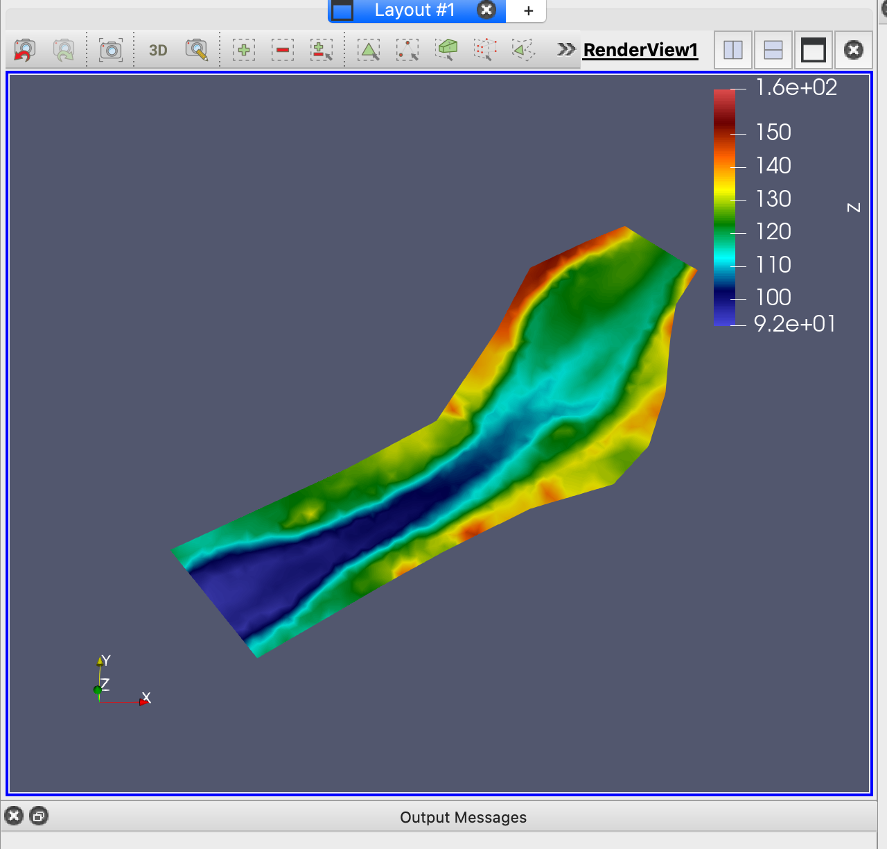
• Select again z in the Variable selector. Note that the color view is smoother due to the interpolation. The result should look as follows:

  

  The 3D appearance is obtained by extruding one of the data variables z or (h+z).

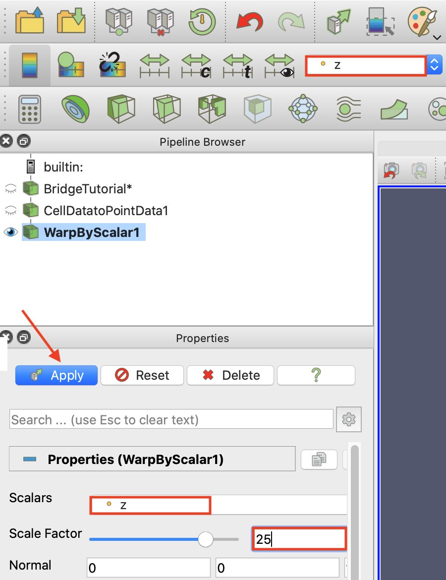
• With the CellDatatoPoint selected in the Pipeline Browser, select Warp by Scalar in the Filters/Alphabetical menu to do the extrusion and then click Apply.

• Configure the Properties tab as follows:

  • Scalars = z

  • Scale Factor = 25

• Click Apply.

• Choose z in the Variable selector.

  

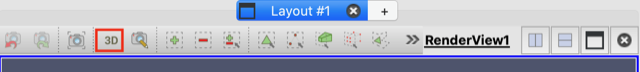
• Switch from 2D to 3D visualization in the Layout Render view to manipulate the project in 3D.

  

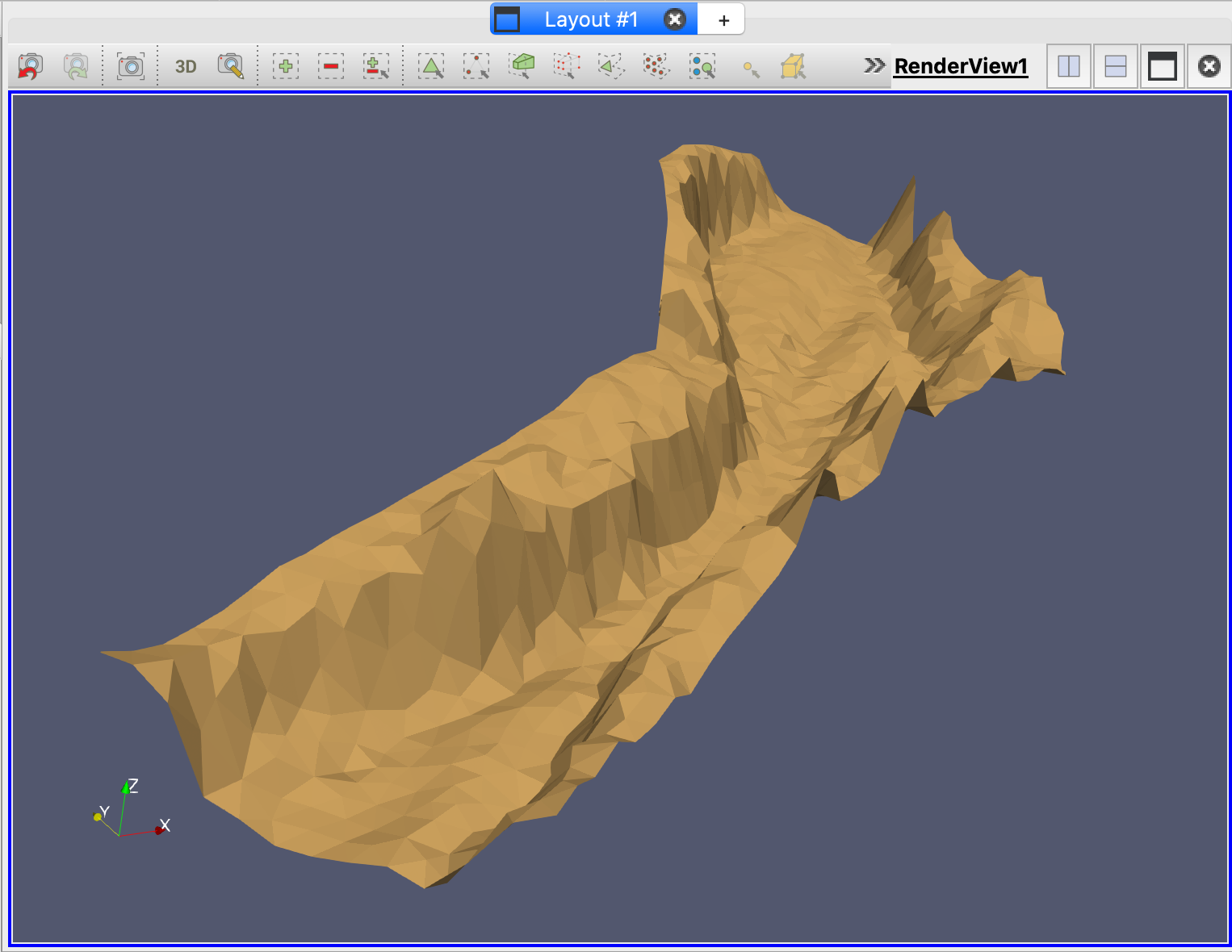
• Remove the color map of the bed elevation z by selecting Solid Color in the Coloring drop-down menu of the Properties tab:

  

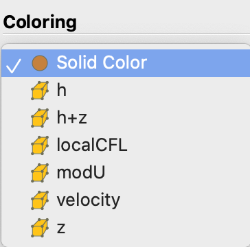
• The Solid Color can be customized clicking the Edit color map icon in the Properties tab. Once the desired color has been chosen at the Pick Solid Color tab (this example uses HTML=#ecb57d), the Render view should look as:

  

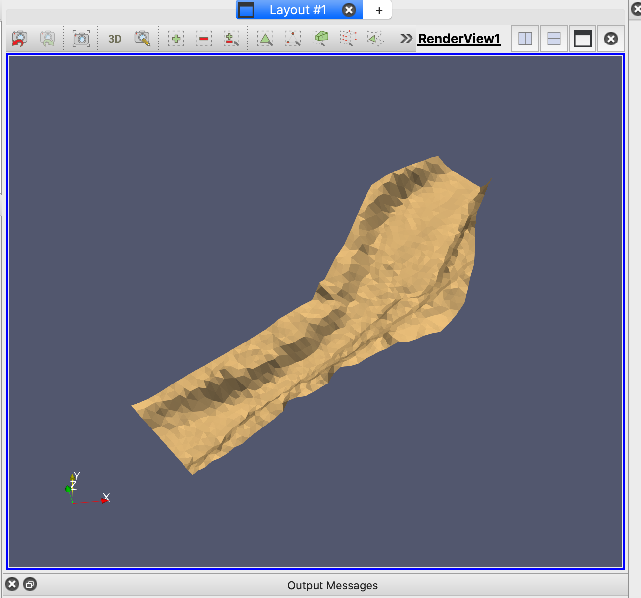
To view the terrain from different points, use the left mouse button to rotate, press down the mouse wheel to translate, and scroll the mouse wheel to zoom in or out the image.

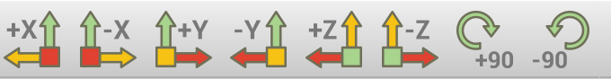
Using the Viewpoint Toolbar (Figure 21.22), you can add different view points of your graphic clicking .

The following image was generated using an alternative view point.

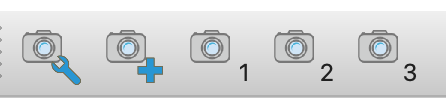
To return to prearranged views use the Camara control toolbar.

A more sophisticated visualization can include additional layers. In the next section we will add two more layers: the water elevation (h+z) and the velocity vector field.

Create a 3D water elevation graphic adding a (h+z) layer

Follow the following steps to create the (h+z) layer:

• Click on the CellDataToPointData item in the Pipeline Browser and select Warp by Scalar in Filter/Alphabetical. A WrapByScalar2 item will be created in the Pipeline Browser.

• Select a time \(\neq 0\) in the Time control toolbar, e.g.

• Configure the Properties panel as follows:

  • Scalars = (h+z)

  • Scale factor = 25 (very important)

• Click the Apply button. Check that h is in the Variable selector.

• Click and choose the Rainbow Desaturated color map, then Apply/Close.

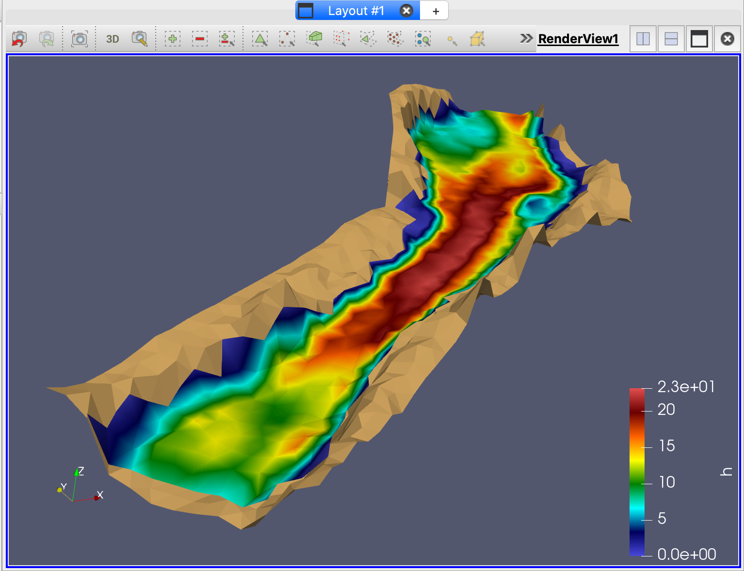
The resulting Render view should look similar to:

As seen in this figure, the layers corresponding to z and (h+z) variables are overlapped in the dry areas of the domain, generating a confusing presentation. One easy way to fix this issue is to remove the water depth h values below a user-defined value to avoid overlapping, doing as follows:

• Click WrapbyScalar2 in the Pipeline Browser and select Threshold in Filter/Common in the main menu

• Click Apply in the Properties panel, and check that h is in the Variable selector.

• Set the minimum value equal to 0.01 m. Depths (h) below this minimum will not appear in the color representation.

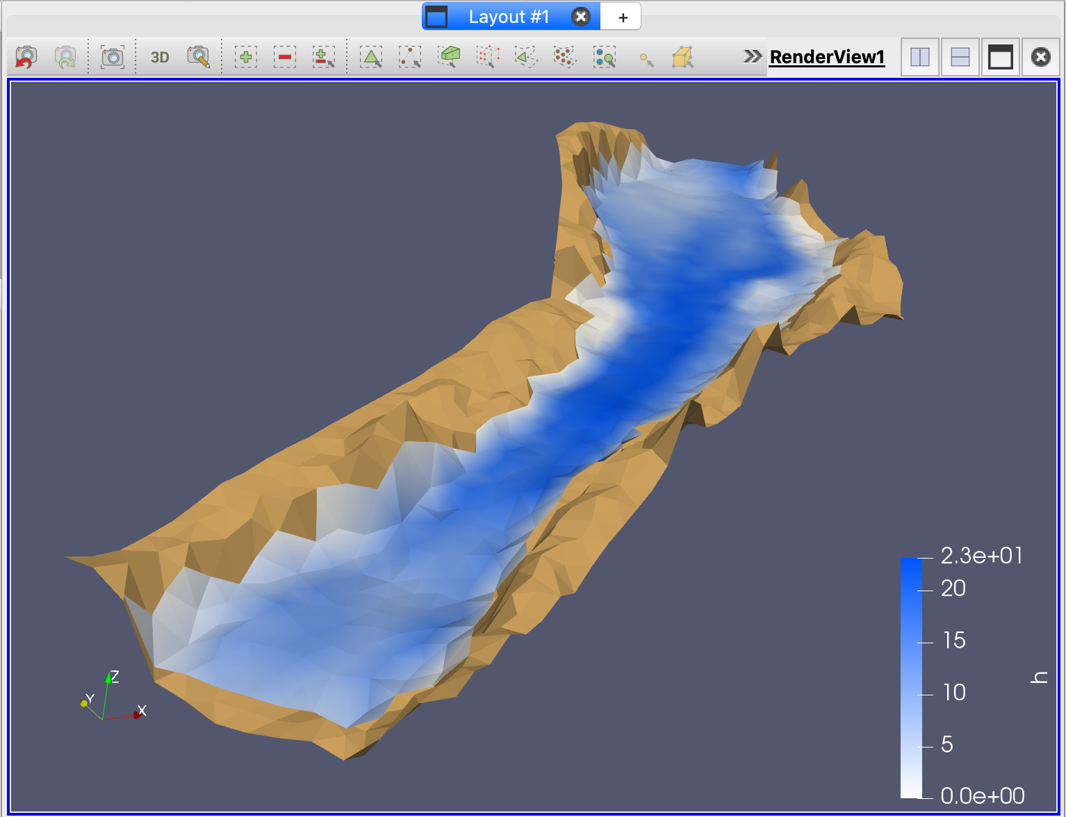
• Click Apply and the result should be as follows:

With the Threshold layer selected, change the color map for water depth h to a white-to-blue as it was explained in Section 21.2.2 of this tutorial. The result graph should look as follows:

Create a velocity field graphic

Follow the following steps to create a velocity field graphic:

• Select the Threshold item in thePipeline Browser.

• In the Filters menu select Common/Glyph and click the Apply.

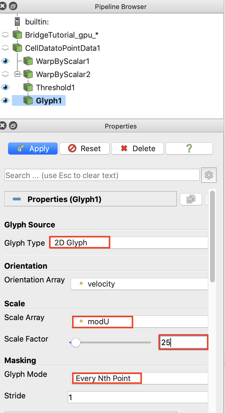
• Configure the Properties panel as follows:

  • Glyph type = 2D Glyph

  • Orientation Array = velocity

  • Scale Array = modU (velocity modulus)

  • Scale Factor = 25

  • Glyph mode = Every Nth Point (to prevent a saturation of arrows in the visualization)

  • Click the Apply button to visualize immediately the filter setup, the user can press this button after each of the previous steps

  • Set Coloring as (modU) for the color map representation and choose the preset color Rainbow desaturated then Apply/Close

  

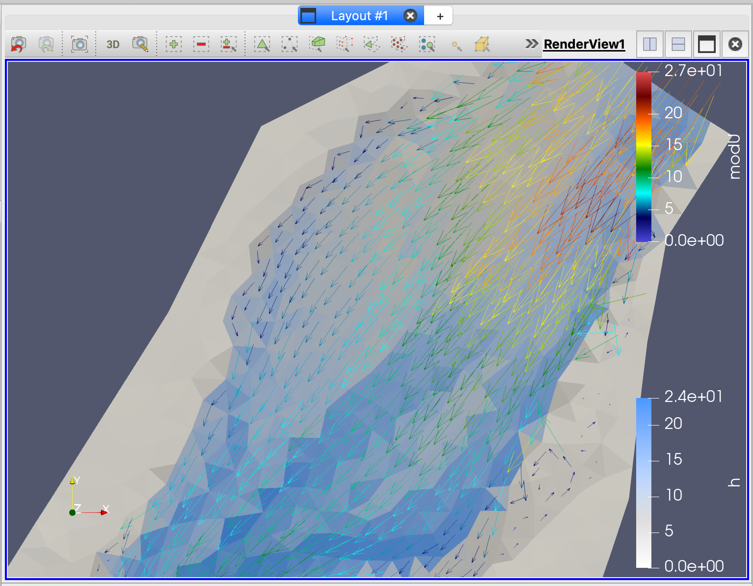
• Select Time \(\neq\) 0 as the current time control tool bar. In this example chose for instance Time=3.

After these steps, the graphic should look like this one:

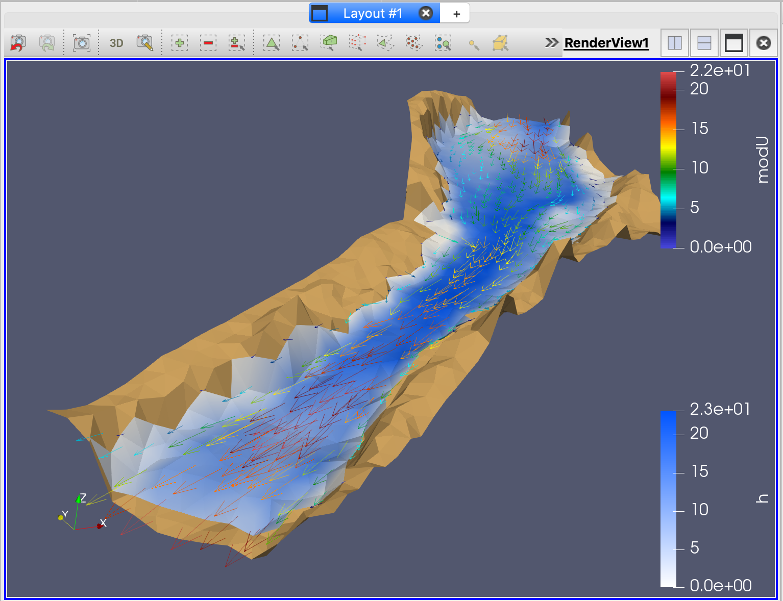
In order to save this Paraview project select File/Save State and create a '.pvsm' file. To load any of the saved projects select emphFile/Load State and select a '.pvsm' file.

Generating animations

With your Paraview project loaded in your computer to create an animation or movie go to File/Save Animation and create a file type '.avi'. The Save Animation Options dialog will be displayed:

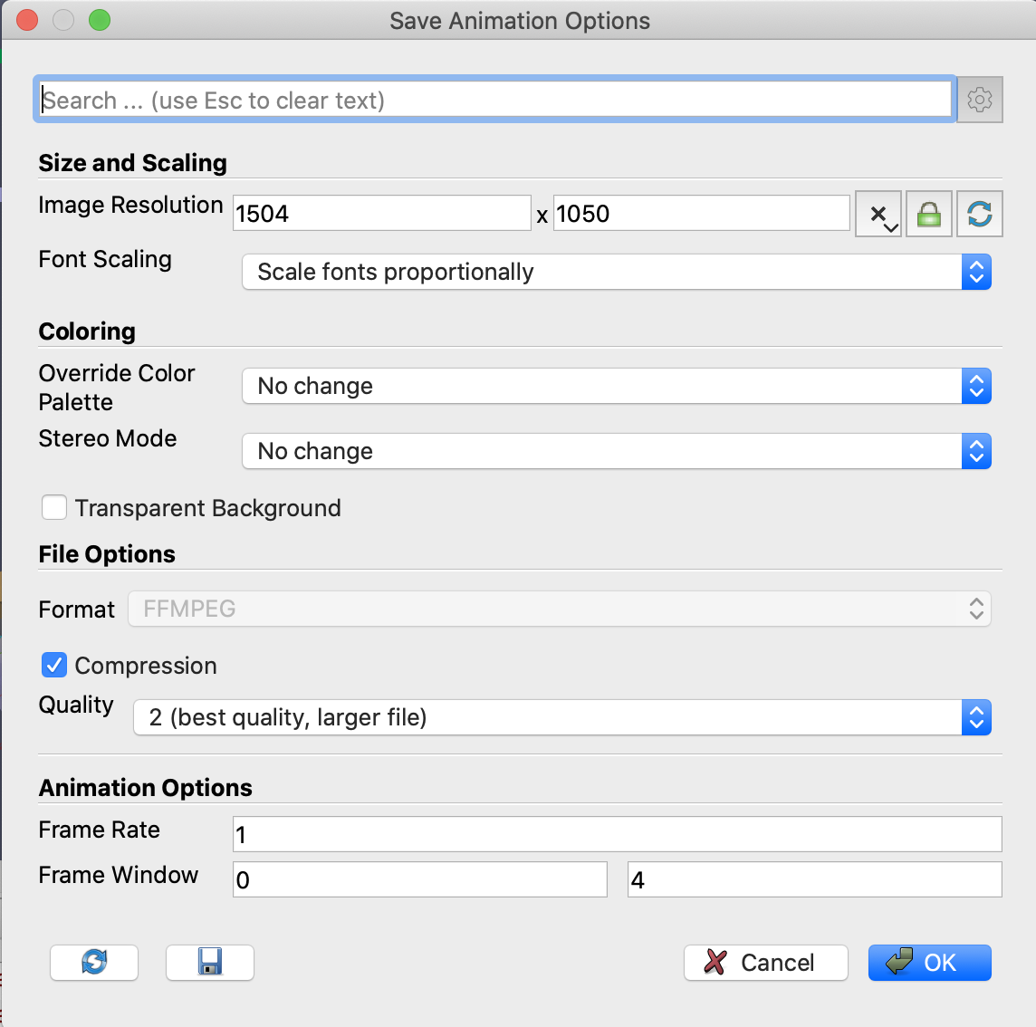
In this dialog, the user can configure the video frame rate, the number of frames per time step, the resolution (in pixels) and the range of time steps. In order to reduce the size of the output video file, a compression mode is also available for the video. Note that this will also reduce the video quality of the animation. As an example, the next figures show three frames of the output video generated in this way, corresponding to six different simulation times.

Animation time frames.

Steamlines representation

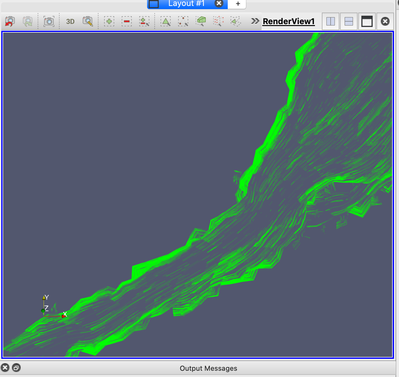
Streamlines represent the instantaneous direction of the velocity and is drawn as unending lines that may converge or diverge from one another. They are drawn at roughly even intervals to capture the flow in all areas.

To create Streamlines with Paraview, follow these steps:

• Open the Paraview application in your computer

• Load the plugin StreamLinesRepresentation in Tools/Manage Plugins in the main menu

• Open the 'BridgeTutorial..vtk' Group file and Select Apply

• Select a time different than 0 in the time control tool bar

• Select velocity in the Variable selector

• In the Properties panel select:

  • Representation = StreamLines

  • Step Length = 1

  • Number of Particles = 1000

  • Max Time to Live = 600

• To have Streamlines in one color, select in the Property panel Coloring = Solid and then click on and select a color.

The next figure shows how the StreamLines look:

If you load a Paraview project '.pvsm' file, you have to deactivate the filters in the Pipeline Browser by clicking the open eyes so that only the '*.vtk' file layer is open.