Simulating a tailings dam failure with RiverFlow2D MT

This tutorial will show how to set up a tailings dam failure simulation with the RiverFlow2D model with the Mud and Tailings Flow Module (MT) using the QGIS interface. The exercise consists of modeling a tailings dam failure flood and creating results maps for the impacted areas. The data is based on the Brumadinho dam disaster occurred on 25 January 2019 when a tailings dam at the CA3rrego do FeijAśo iron ore mine, east of Brumadinho town, in Minas Gerais, Brazil, suffered a catastrophic failure.

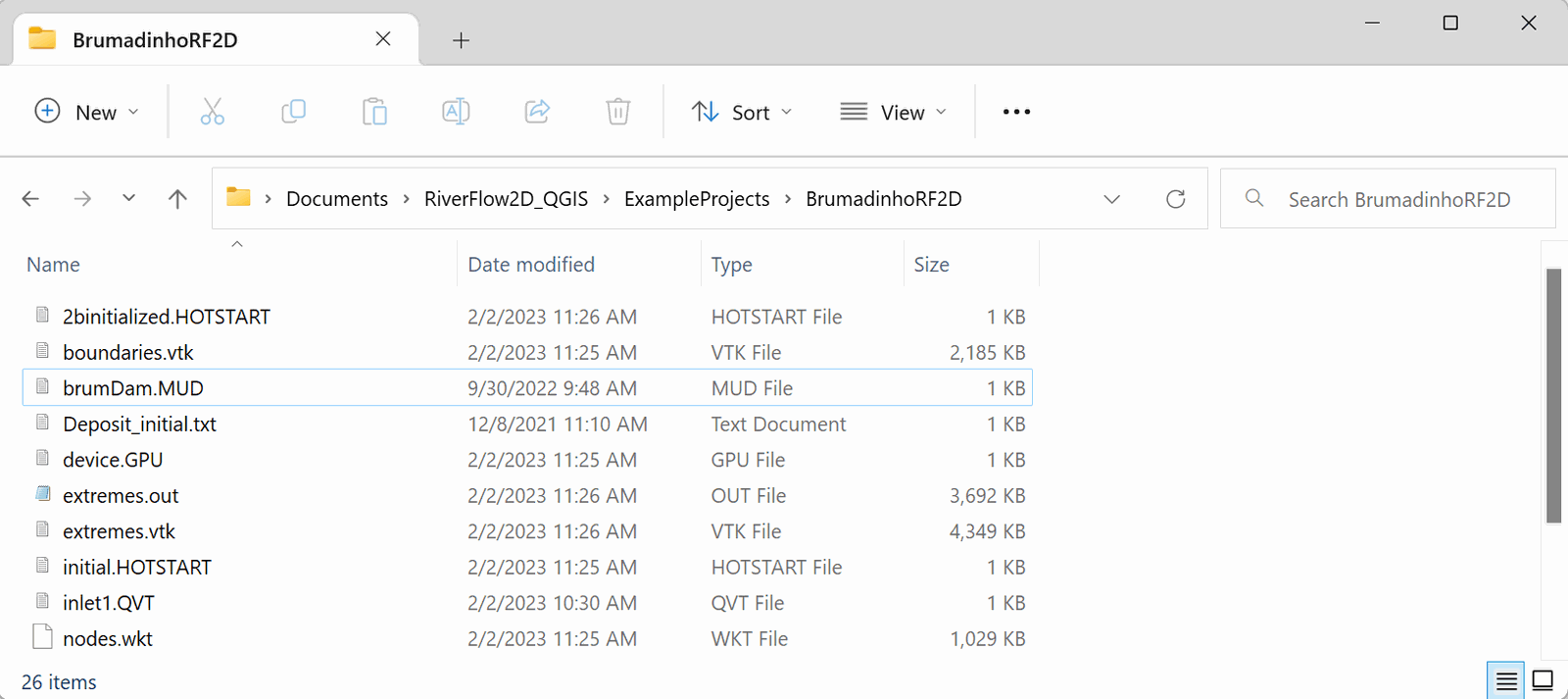
::: shaded The files required to follow this tutorial can be extracted from the 'ExampleProjects' zip file under the 'BrumadinhoRF2D' folder. This zip file is downloaded separately from your installation materials. :::

Start a new project for a tailing dam break simulation

1. To create a new RiverFlow2D project, open QGIS and click on the New RiverFlow2D Project button in the toolbar. A dialog window appears where you select the layers that will be created, the name of the Senario, the Coordinate Reference System (CRS), and the directory path where the layers will be saved. This example will use the layers: Domain Outline, Manning N, BoundaryConditions, MeshDensityLine, and InitialConcentrations.

2. Select None in the Layers drop-down menu, then click the MeshDensityLine and the Initial Concentrations check boxes.

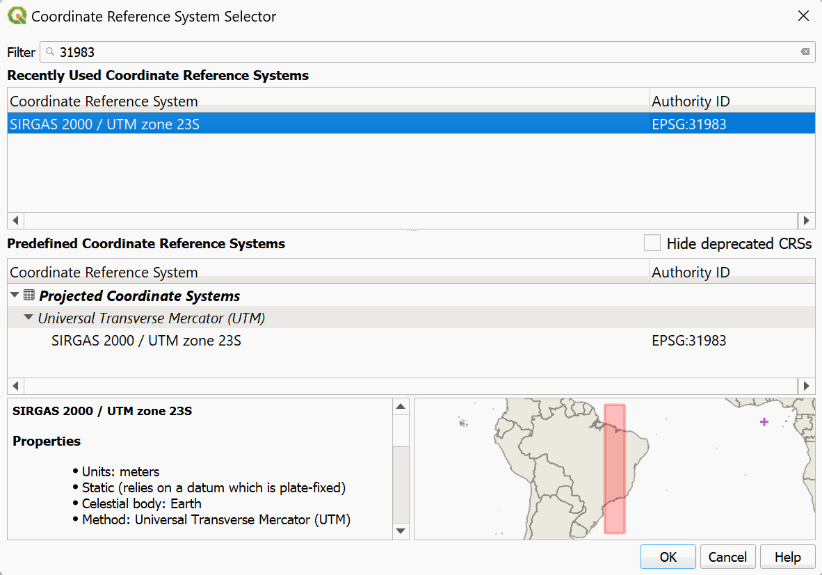
3. Click the Projection button and in the Filter text box, type 31983 and select the Coordinate Reference System and click OK as shown:

   

4. Click the button to provide a path to store the project files in the Project Directory text box. This will be the folder where the model will write all results and output files. Browse to the tutorial directory in the location where the files were extracted, in the 'BrumadinhoRF2D' folder, then click Select folder. The dialog window should look like the following:

   

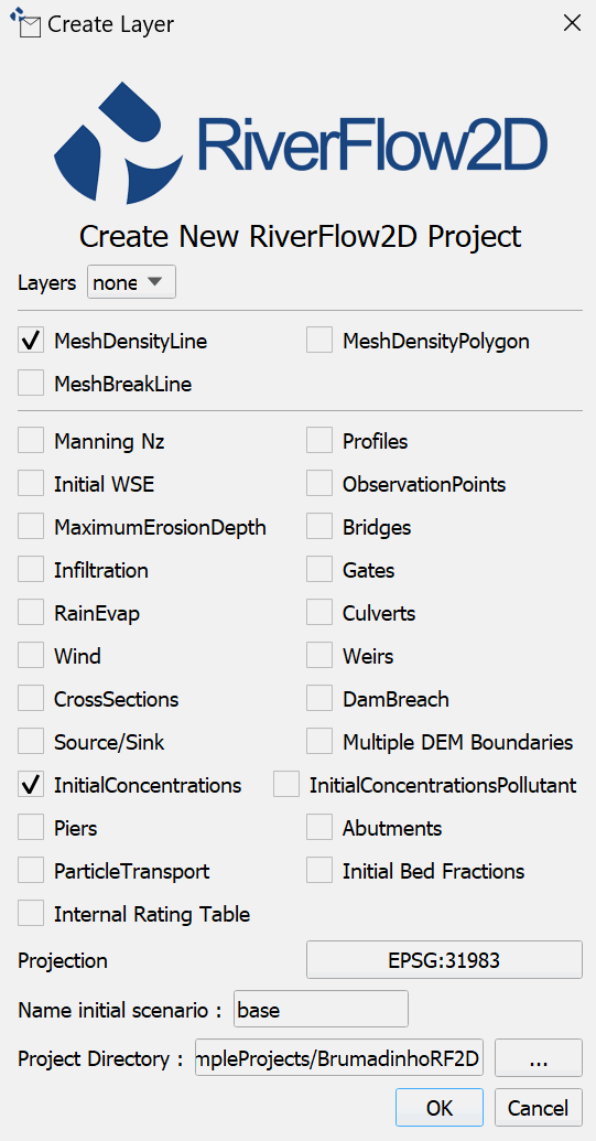
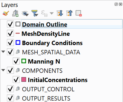
5. After clicking OK, the layer templates are created, and displayed on the Layers Panel

   

   ::: shaded On the QGIS Project menu, click Save, to save the project in the same directory that you previously selected in the Create New Project dialog above. :::

Load elevation data

In this tutorial we will use two Digital Elevation Model or DEM raster files that contain the terrain elevation data and tailings dam volume data.

1. To load the DEMs, click the Add Raster Layer button . You may also use the QGIS shortcut Control+Shift+R.

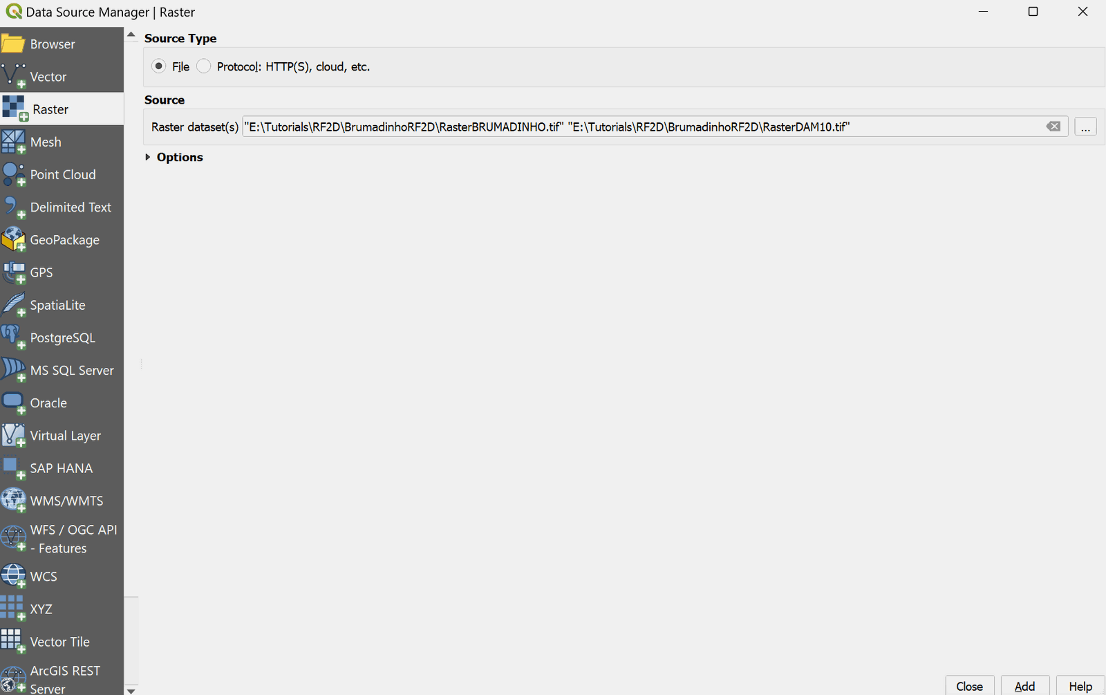
2. In the dialog search for the tutorial folder and select the 'RasterBRUMADINHO.tif' and 'RasterDAM10.tif' files as shown:

   

3. Click Add and then Close.

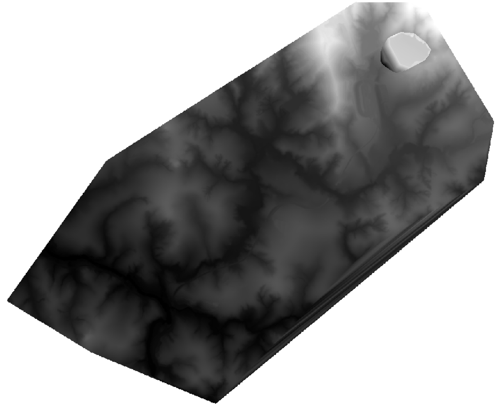
4. Click on the RasterBRUMADINHO layer. Use the Zoom to Layer button to center the image.

   The raster will be displayed on the screen, by default it is rendered in gray gradient as shown.

   

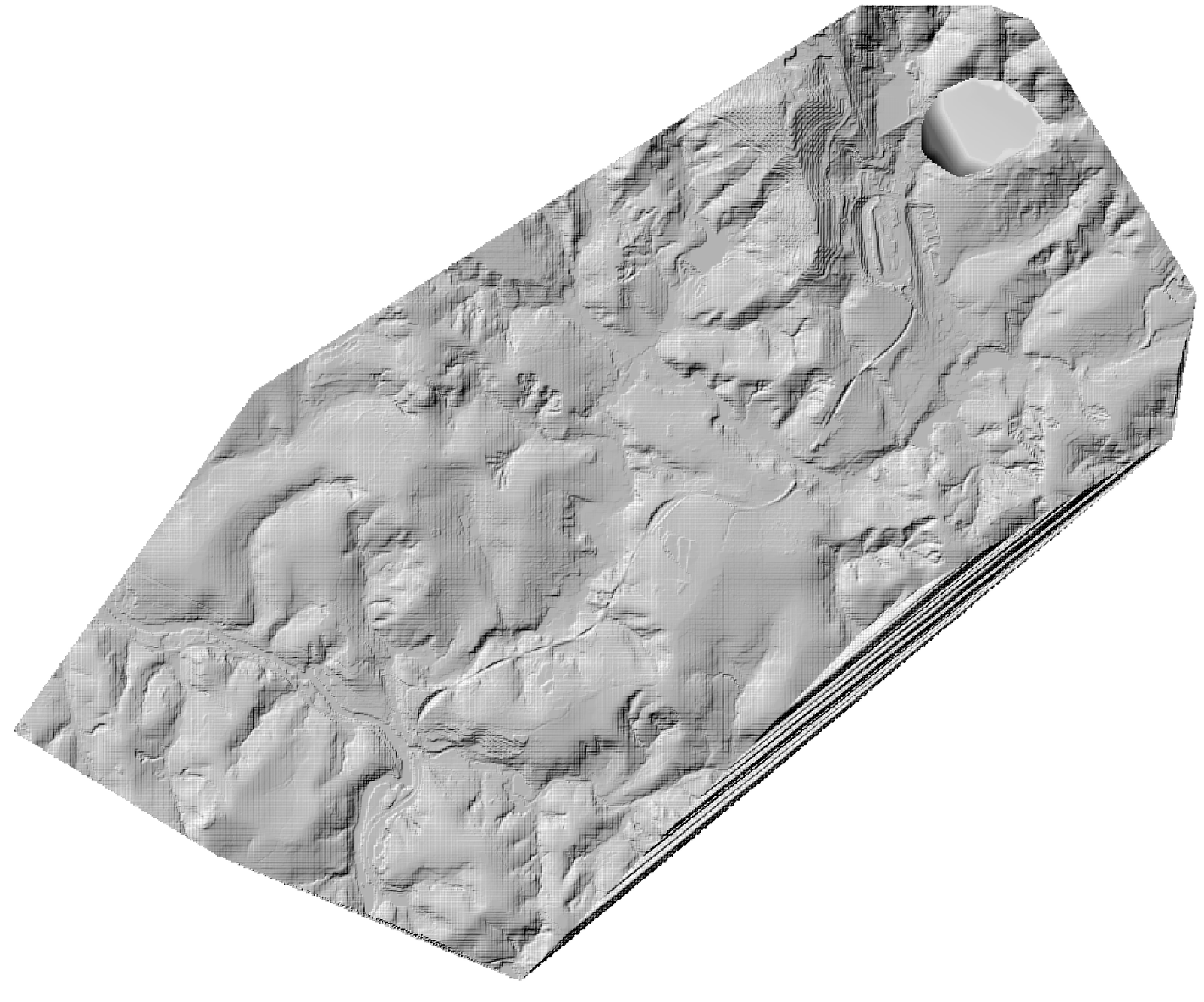
   Right-clicking on the label of the new raster layer and selecting Properties, in the Symbology panel you can change the Render type for a more informative palette such as Hillshade for instance.

   

::: shaded You may move the raster layer by dragging it to the end of the list of layers to avoid that it would hide or interfere visually with the other layers. :::

Create the limits of the modeling area

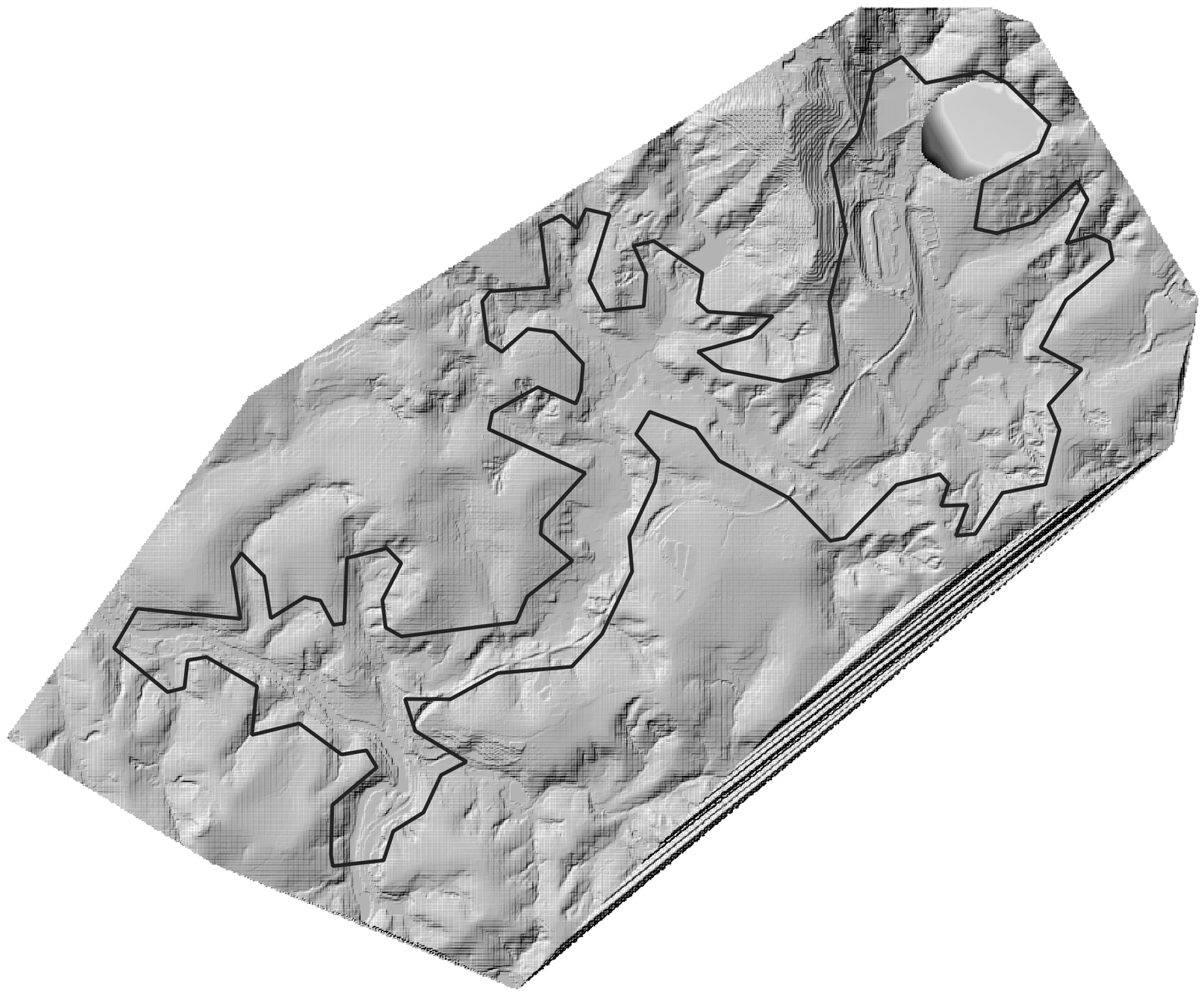
We define the limits of the modeling area drawing a polygon on the Domain Outline layer. To create it do as follows:

1. Click the Domain Outline layer to activate it and then click Toggle Editing (pencil) in the toolbar

2. Click the Add Polygon Feature tool . Proceed to delineate the outline of the polygon by clicking the vertices with the left mouse button.

3. To finalize and close the polygon, right-click on the map view area. A dialog window to input the cell size attribute of the newly created polygon will appear. The CellSize value for the reference size of the mesh cell is indicated. Enter a value of 50 m.

   The Domain Outline should look similar to the following figure:

   

4. Save the polygon by clicking the Save Layer Edits button .

5. Click on Toggle Editing button to deactivate the layer Edit mode

Create more detail for the mesh down the main flow area

Once the Domain Outline is created, a Mesh Density Line will provide the necessary detail down the main channel for more accuracy.

1. Select the MeshDensityLine layer making sure it is activated as shown

   

   and click the Toggle Editing button .

2. Click the Add Line Feature button then Left-click to draw the points down the middle of the channel all the way to the river entrance at the bottom of the Domain Outline.

3. Right-click to finish the line. A dialog requesting input for the MeshDensityLine Feature Attributes will appear. Input 25 as the CellSize for the MeshDensityLine layer. The first line should look as follows:

   

   Another line will need to be drawn to finish adding detail down the main path on the river in the south.

4. Click the Add Line Feature button then Left-click to draw the points starting from the the south-western part of the Domain Outline along the riverbed and right-click to finish the line, joining it to the first line as follows: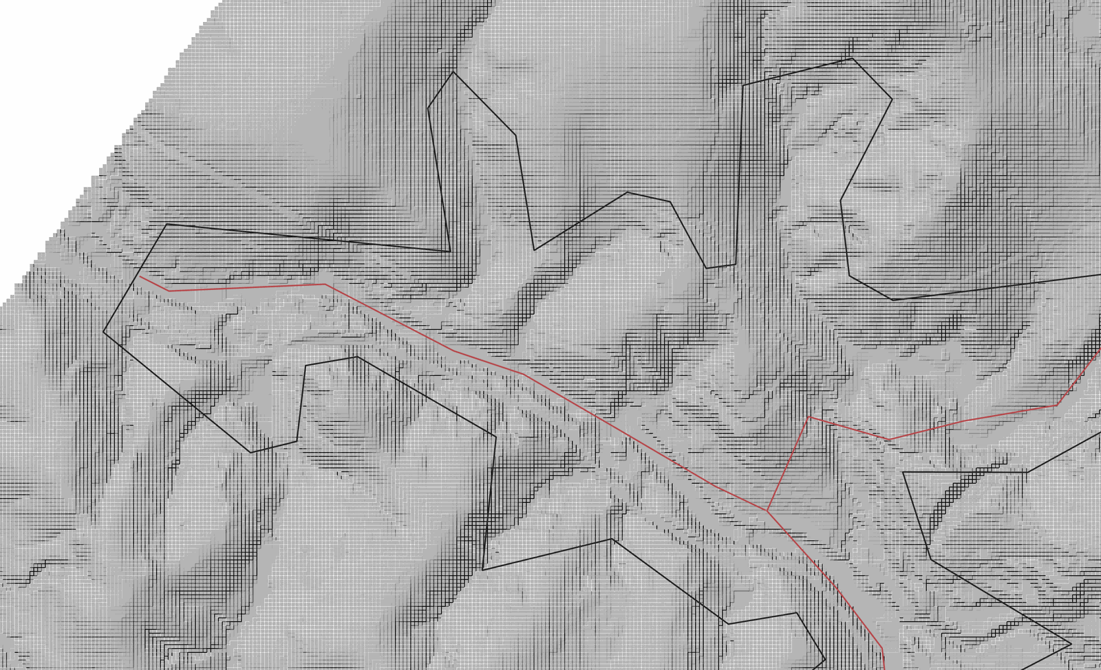

   

5. Right-click to finish the second line. A dialog requesting input for the MeshDensityLine Feature Attributes will appear. Input 25 as the CellSize for the MeshDensityLine layer.

6. Save the polygon by clicking the Save Layer Edits button .

7. Click on Toggle Editing button to deactivate the layer Edit mode

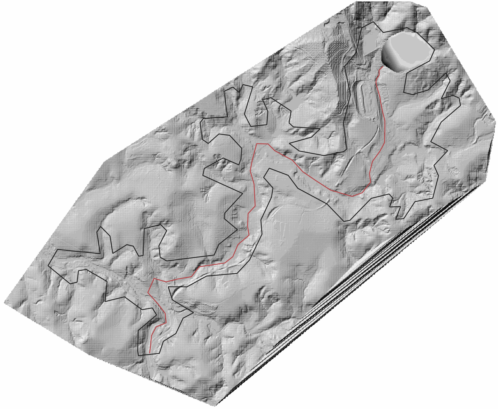
   The finished MeshDensityLine layer should look as follows:

   

Generating the triangular-cell mesh

Now that the Domain Outline and Mesh Density Line layer have been created, proceed to generate the mesh by clicking on the Generate Trimesh button.

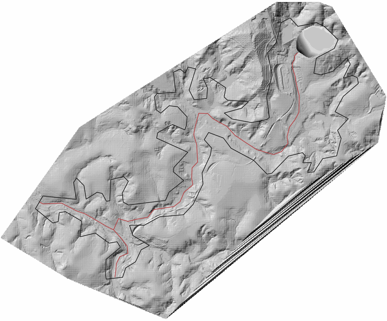
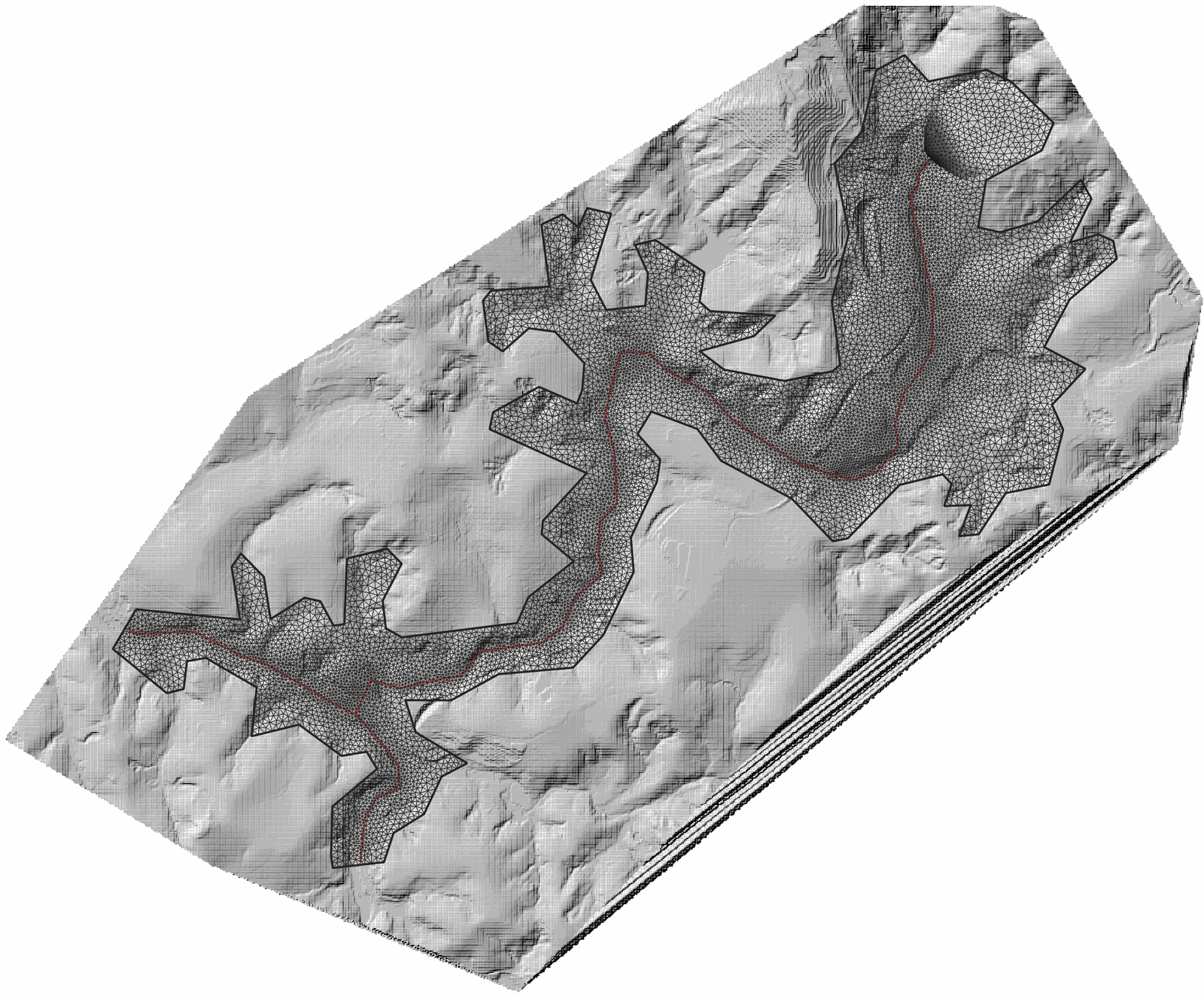
The following figure shows the generated mesh. You will also see in the Layers panel the new layer: Trimesh

Setting up the boundary conditions

Here we will explain how to enter boundary conditions that are needed in any inflow or outflow sections of the model area where flow can enter or leave the mesh. In this tutorial we will have one inflow and one outflow condition.

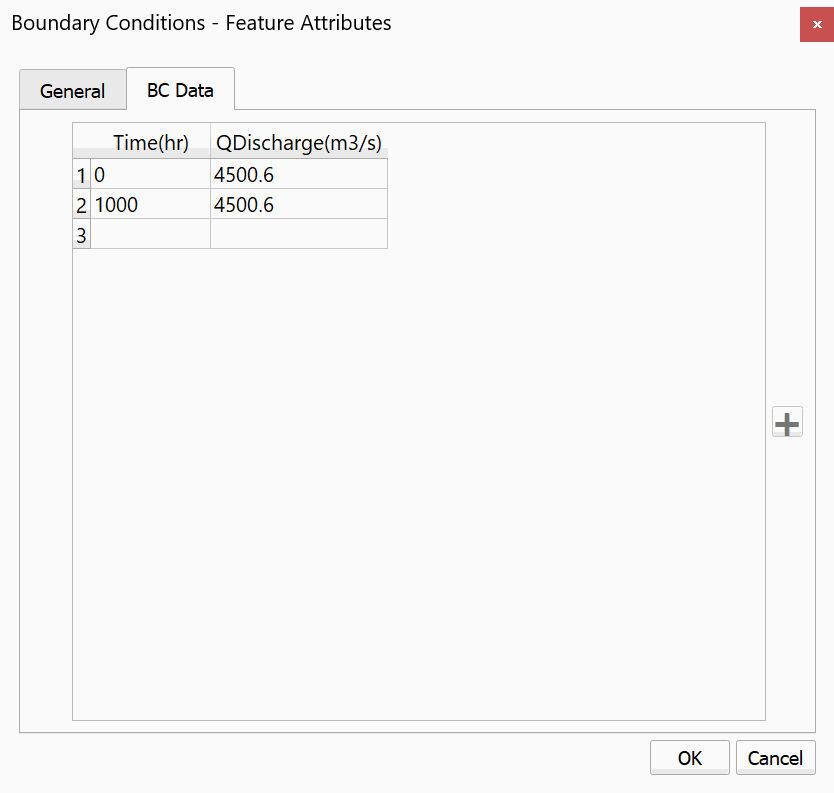
We first enter the inflow boundary condition imposing a hydrograph (discharge vs time).

1. Select the BoundaryConditions layer in the Layers panel.

2. Click the Toggle Editing button to add the polygons that will indicate the open boundary segments where inflow and outflow conditions are imposed. Draw a polygon at the bottom end of the mesh as indicated in the figure: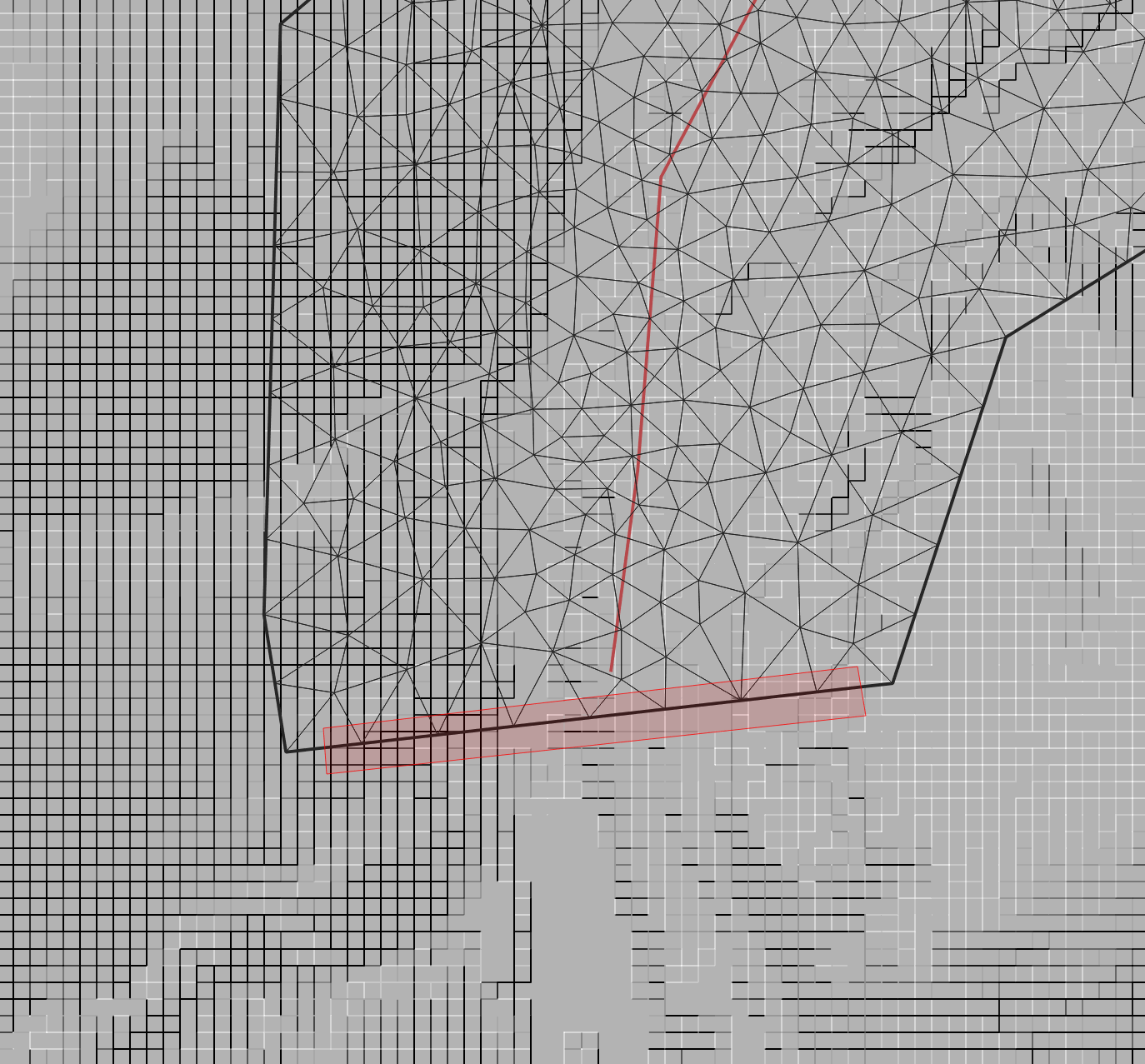

   

3. To finish the polygon, right-click on desired location. A window to enter the attributes of the newly created polygon is displayed.

   ::: shaded The exact form of the polygon is not important. You only need to make sure that the polygon covers the segment length at which you want to impose the condition. All cells falling within that polygon will be open boundary cells. :::

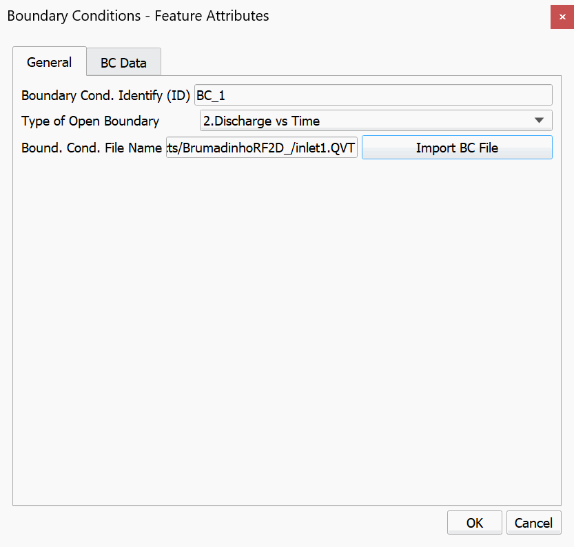
4. In the Boundary Cond. ID enter the desired name or leave the default.

5. Select 2. Discharge vs. Time from the Type of Open Boundary list.

6. Click Import BC File button, and search for the 'inlet1.QVT' hydrograph file as shown below:

   

   

7. Click OK to close the dialog and then click Save Layer Edits .

::: shaded All boundary condition files, such as 'inlet1.QVT' in this tutorial, need to be in the same directory as all the other project files. :::

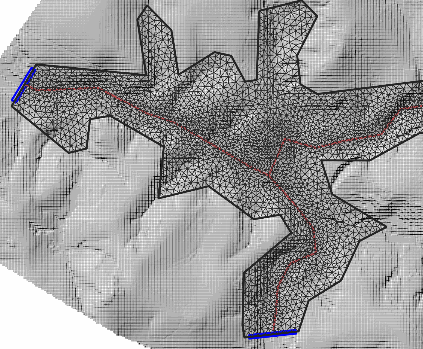
Now we will enter an free outflow condition where the fluid will be let to flow out from the mesh.

1. Click the Add Polygon Feature tool . Proceed to delineate the outline of the polygon by clicking the vertices with the left mouse button. Draw the polygon defining the outflow boundary area at the downstream end of the river as shown: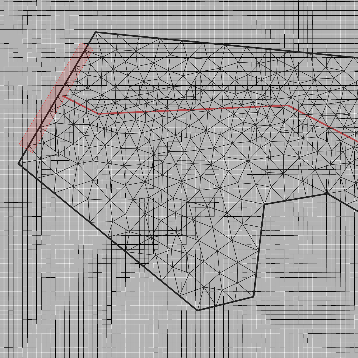

   

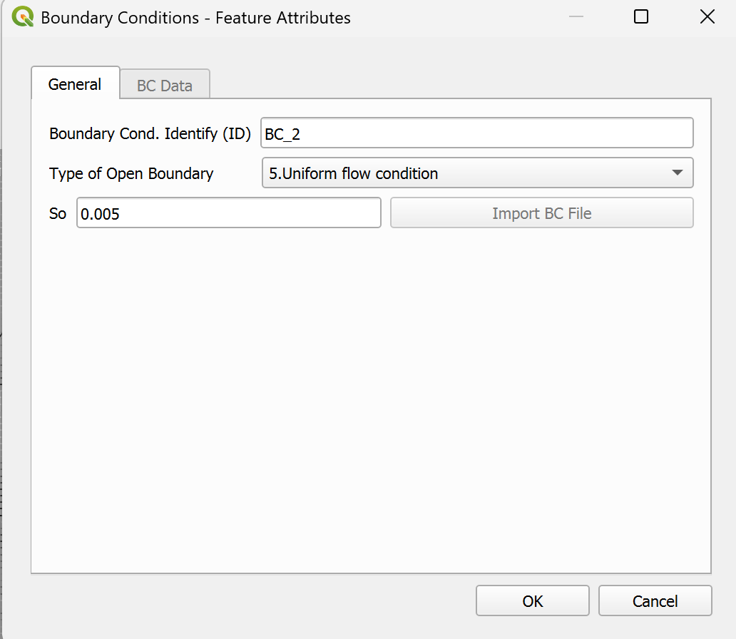
2. Right click to close the polygon. A dialog window will appear to enter the parameters. Select the condition type Uniform flow condition and set So to 0.005. The dialog should look like the following:

   

3. Save the changes made to the layer by clicking the Save Layer Edits button .

4. Deactivate editing mode by clicking on the Toggle Editing button .

   The figure below shows how the BoundaryConditions layer should look:

   

Assigning Manning's n

Manning's n is the parameter determining the bed roughness. The model requires that all cells in the model area have a defined n. In a project application we should have n's that vary through the mesh since variable vegetation and terrain characteristics will have different roughness. However, for simplicity, in this tutorial we will assume a single n.

1. Select the Manning N layer and click the Toggle Editing button .

2. Click the Add Polygon Feature to draw a polygon that covers the entire domain. The polygon may extend beyond the mesh area as shown: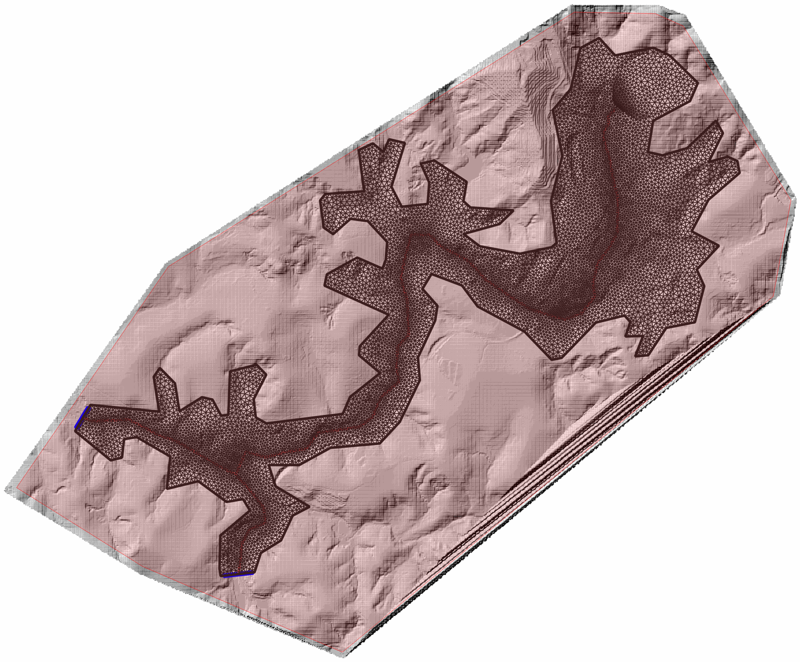

   

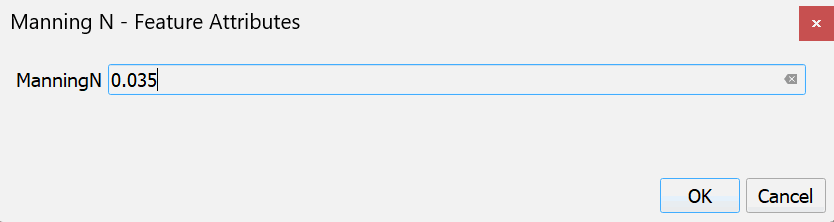
3. Close the polygon by right-clicking on the end vertex and enter a Manning's n equal to 0.035:

   

4. Click Save Layer Edits , and then click the Toggle Editing button to deactivate editing mode.

Providing the Initial Concentrations for the tailings material

The RiverFlow2D MT model allows defining initial volume concentrations that vary in space. In order for the model to assign this initial state, one or more polygons must be drawn over the tailings raster or initial water surface elevation polygon. This polygon will then be assigned a data table attribute that gives the concentrations for each sediment class.

1. Select the InitialConcentrations layer in the Layers and click the Toggle Editing button

2. Click the Add Polygon Feature button and draw the polygon, keeping within the edges of the RasterDAM10 raster: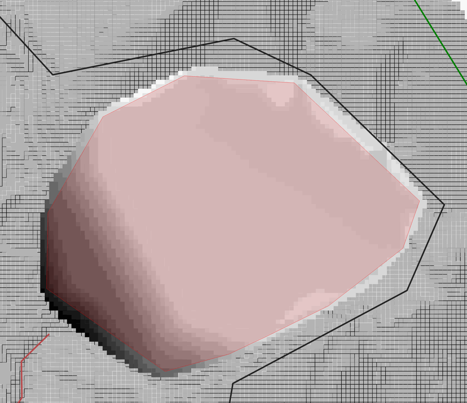

   

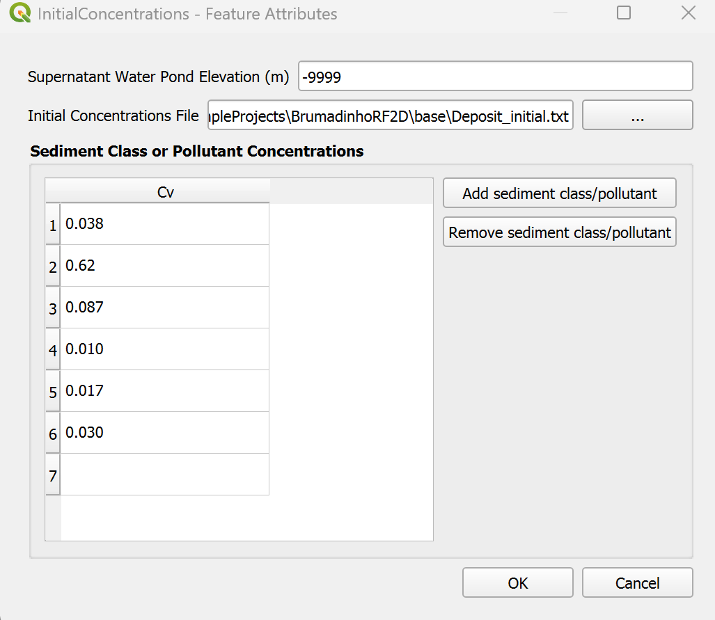
3. An InitialConcentrations - Feature Attributes dialog will appear. On the Initial Concentrations File line click the Browse button to select the 'Deposit_Initial.txt' file from the project folder '\ExampleProjects\BrumadinhoRF2D\base\' folder and then click OK.

4. The dialog should look like the following:

   

5. Save the changes made to the layer by clicking the Save Layer Edits button .

6. Click the Toggle Editing button to disable editing mode.

::: shaded Save the QGIS project using the Save Project button or by using the Project menu. Name the project file 'Brumadinho.qgs'. :::

Exporting the project from QGIS to RiverFlow2D

Once the layers with the input data to the model have been created, we need to export data files required to run RiverFlow2D.

1. In the RiverFlow2D plugin toolbar, click the Export files for RiverFlow2D button and select Export RiverFlow2D ...

2. In the export dialog window indicate the Project Name, Brumadinho in this tutorial.

3. In the drop-down menu for DEM Single Raster select RasterBRUMADINHO

4. Click on the Options arrowhead to view the additional parameters for the export.

5. under DEM (Single Raster) make sure RasterBRUMADINHO is selected in the dropdown menu.

6. Click to enable the checkbox for Using Initial WSE Raster Layer, then on the drop down menu select the RasterDAM10 as your InitialWSE layer.

   Your Export RiverFlow2D dialog window should look like this:

   

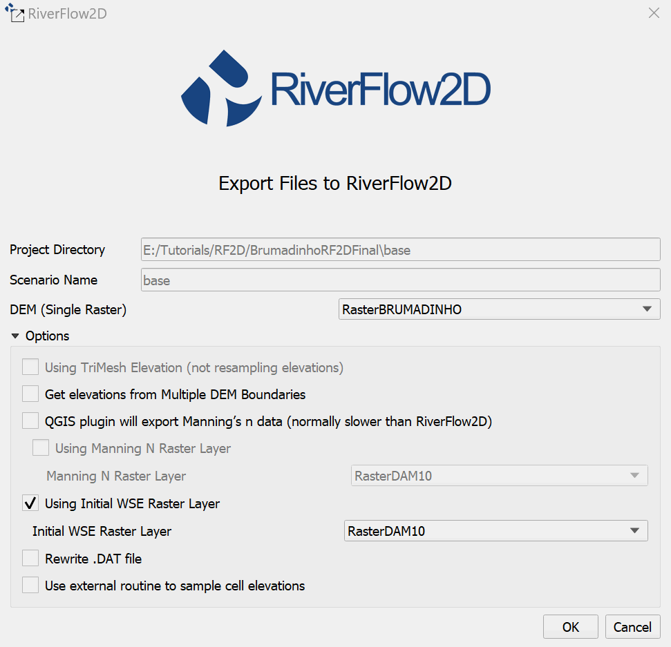
7. Click OK.

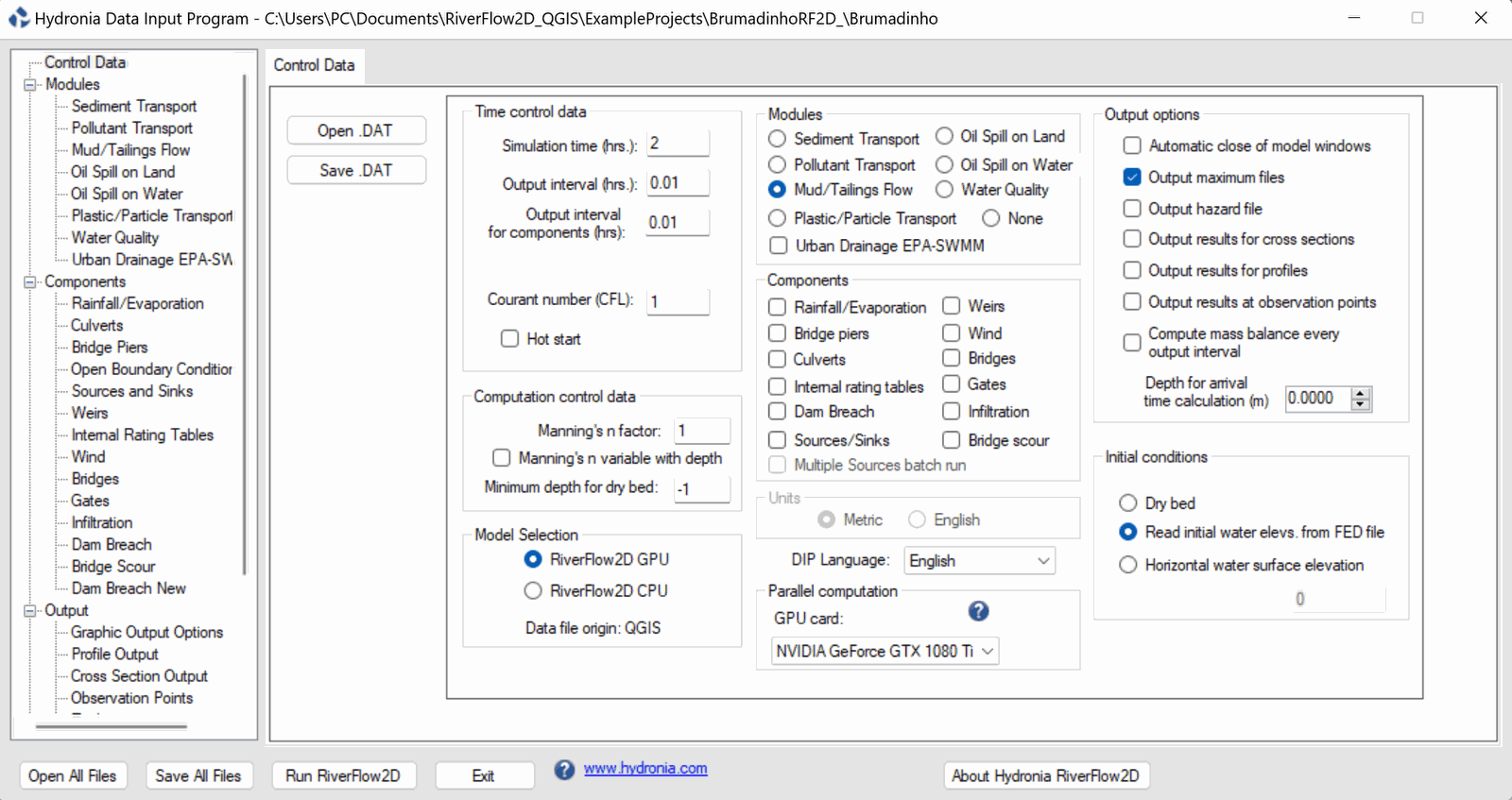
Configure final model parameters in the Hydronia Data Input Program [(]{.nodecor}DIP[)]{.nodecor}.

Once the model files have been created, the Hydronia Data Input Program will appear automatically with the main control data file loaded, in this case: 'Brumadinho.DAT'.

Control Data Panel

The following parameters will need to be changed as indicated:

1. In the Control Data panel under the Time control data section, Set the Output interval [(]{.nodecor}hrs.[)]{.nodecor}: to 0.01.

2. In the Modules section click the Mud/Tailings Flow radial button.

   ::: shaded *Optional* If you have an nVidia graphics card installed on the system, you can enable the RiverFlow2D GPU under the Model Selection section to accelerate the computation speed for the simulation. :::

   The Control Data panel should look like the following:

   

3. Click the Save .DAT button. Click Save again in the dialog box and click Yes to replace the existing file.

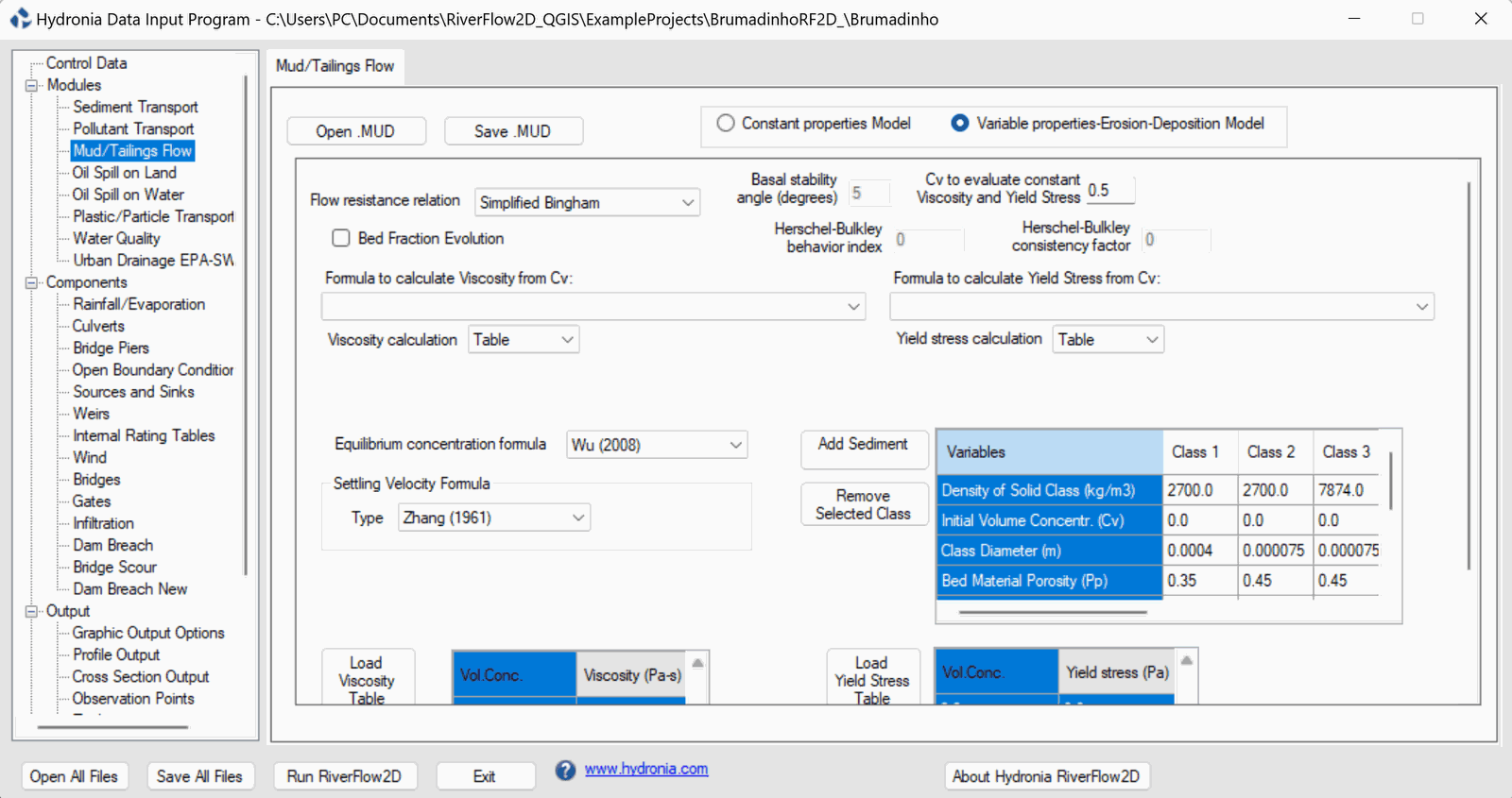
Mud/Tailings Flow Panel

The Mud/Tailings Flow module needs to be configured with the tailings properties and other rheological parameters. Please do the following:

1. Click on the Mud/Tailings Flow on the left side panel to activate it.

2. In the Mud/Tailings Flow panel, click the Open .MUD button.

3. A dialog will appear asking for a file ending with the '.MUD' extension. Browse for the file '\ExampleProjects\BrumadinhoRF2D\base\brumDam.MUD' and click Open.

   You will now see that the panel has changed most of the parameters. More importantly, the Variable properties-Erosion-Deposition Model has been enabled, and there are six sediment classes loaded. Take some time to familiarize yourself with the parameters.

   The parameters that have been loaded need to be saved with the same name as the project name so that the model will use it upon execution.

4. Click the Save .MUD button and the Scenario name 'base.MUD' should already be set. Click Save.

   The Mud/Tailings Flow panel should look like the following:

   

   Providing the Viscosity and Yield Stress data for Variable properties-Erosion-Deposition Model

   When selecting to use the Variable properties-Erosion-Deposition Model in this tutorial, data tables for the volume concentrations relationship with Viscosity and Yield Stress need to be provided. These files are already prepared for this tutorial, and must be copied into the Scenario folder as follows:

   1. In File Explorer browse to the location of the project folder '\ExampleProjects\BrumadinhoRF2D\'

   2. Select the following files from the folder: 'YieldStressVsCv3.txt, ViscosityVsCv3.txt'

   3. Copy the files into the Scenario folder '\ExampleProjects\BrumadinhoRF2D\base\'

   Updating the Inflow Boundary Condition File

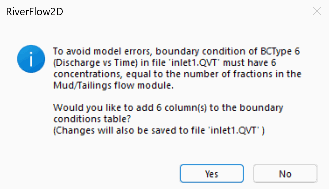
   It is critical to update the Open Boundary Conditions data file with additional columns of data that represent the new sediment classes. By default this file contains a table of time and discharges, but the model requires for all inflow conditions the volume concentration for each sediment or material class. In case of water flow, all concentrations must be set to 1. To update it do the following:

5. Click on the Open Boundary Conditions under Components in the side panel of the Hydronia Data Input Program.

6. Click on the cell in the first table that contains the 'inlet1.QVT' variable:

   

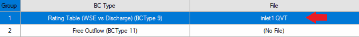
   Upon clicking the cell, a dialog box should appear that will allow us to automatically update the existing data table in the 'inlet1.QVT' file with the additional rows needed, and setting each to 0:

   

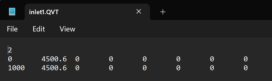
7. Click Yes to update the 'inlet1.QVT' file.

   You can verify the contents have been updated by scrolling to the right in the file contents section or by opening the '\ExampleProjects\BrumadinhoRF2D\base\inlet1.QVT' file in Windows Explorer. Your Inlet1.QVT file should look like the following figure:

   

Running the model

The simulation is now ready to run. Proceed as follows:

1. Click on Control Data in the side panel of the DIP and then click the Run RiverFlow2D button at the bottom.

2. The DIP will ask to save changes to the .DAT file, click No.

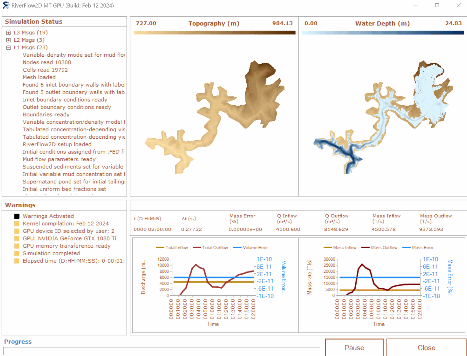
   A few windows should appear, the last one will be the graphical model windows that displays the status of the model. When the model is finished running, it should look as follows:

   

3. Click Close and let the program finish writing the remaining output files.

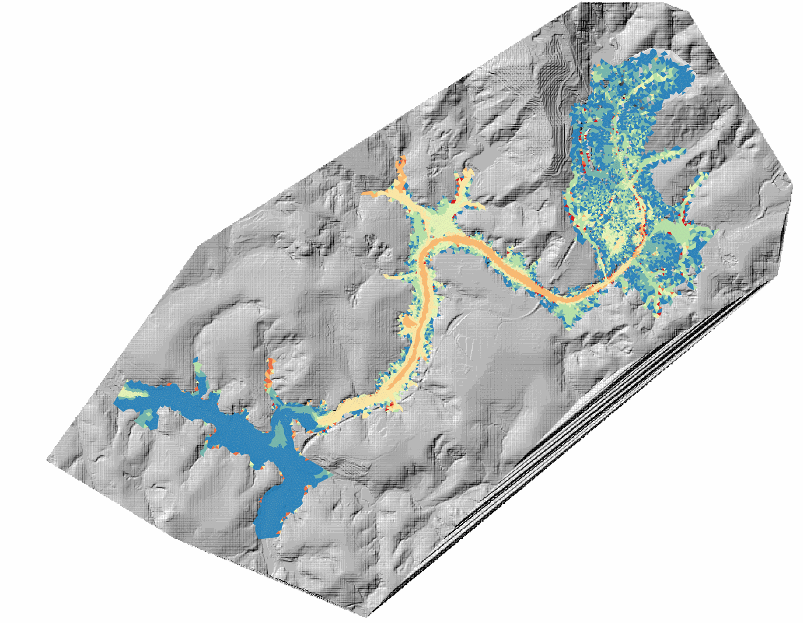
Generating maps for the Mud/Tailings Flow module

Once the model has finished running we can create maps for various outputs. This tutorial will focus on some of the specific maps that can be generated once the Mud/Tailings module with variable properties-erosion deposition enabled.

1. In QGIS , in the RiverFlow2D plugin toolbar, click on the drop down menu for Results vs Time Maps and select Concentrations and Properties vs Time Maps

   

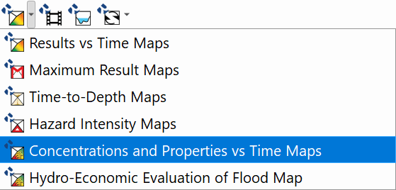
   The Concentrations and Properties vs Time Maps window will provide maps for each Sediment class, labeled Conc_# under the Maps subsection. Users can also create maps for each of the variables in the list.

2. Select one of the Maps, then select an Output Times of interest. You can hold Control key while clicking on multiple Maps and / or Output Times.

3. Once all outputs of interest are selected, click on the Right Arrow button to move them to the Output Maps subsection.

   

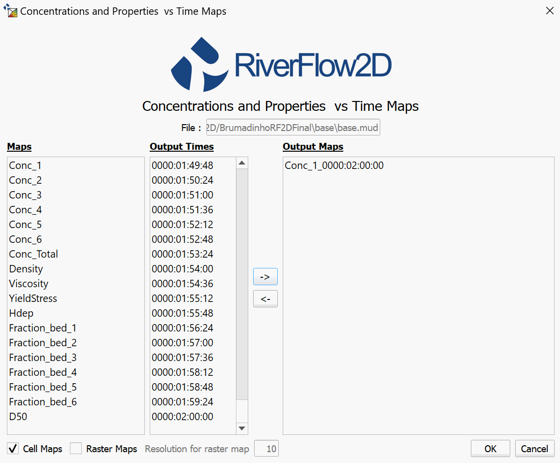
4. Click the OK button to generate the maps.

   The Layers panel on the left side will have a group named OUTPUT RESULTS where the resultant map or maps will be placed.

Repeat these steps to create maps for each of the concentrations if desired.

Generating animations for the Mud/Tailings Flow module

An animation can best illustrate the mud / tailings flow over time. This section will show how to generate results for the specific variable properties-erosion deposition enabled model outputs.

::: shaded On the QGIS Project menu, click Save, to save the project in the same directory that you previously selected in the Create New Project dialog above. This is required for the Animations panel to function. :::

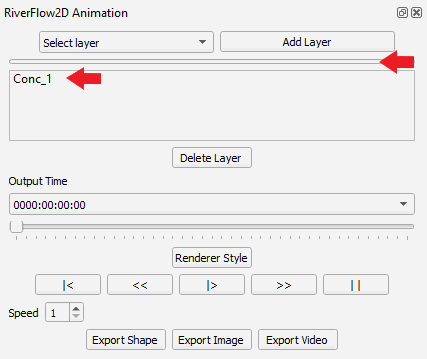
1. Start by activating the Animations panel in the RiverFlow2D plugins toolbar

   A panel will appear below the Layers panel on the bottom left.

2. Click on the Select layer drop-down menu and select Mud/Tailings Flow.

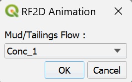
3. Click Add Layer. A dialog box will appear asking for the specific Animation we would like to create:

   

4. Click on the drop-down menu to see the available outputs. They will be the same as the ones from Concentrations and Properties vs Time Maps plugin.

5. Choose any of these and click OK.

6. Select the output range desired, or just leave the default for the entire range of output intervals. Click OK

   There is a status bar underneath the Select layer drop-down showing the progress of the animation generation. When it is finished, the layer previous choice of animation will appear in the box underneath the status bar.

   

7. Click and hold to drag the newly created ANIMATION group in the Layers panel and move it above the Raster layers so that the animation will be visible.

8. Click on the layer that was generated in the RiverFlow2D Animation panel then click the Play button to view the animation.

   Repeat these steps to create animations for each of the concentrations if desired.

This concludes the tutorial for Simulating tailings dam Failures utilizing the Mud/Tailings Flow module in RiverFlow2D.